Bayesian synthetic control workflow#
The synthetic control method is one of the most influential innovations in causal inference for policy evaluation [Athey and Imbens, 2017]. This notebook demonstrates the full workflow — not just model fitting, but the recommended pipeline of feasibility assessment, estimation, and validation recommended by Abadie [2021], augmented with Bayesian design tools from the geo-experiment literature [Brodersen et al., 2015, Meta Incubator, 2022].
We use the California Proposition 99 dataset — the canonical example from the SC literature. In 1988, California passed Proposition 99, which imposed a 25-cent tax on cigarette packs. Abadie et al. [2010] estimated the causal effect of this policy on per-capita cigarette sales using the remaining 38 US states as a donor pool. This example is ideal for demonstrating the workflow because the treatment effect is large, sustained, and well-documented.
Before the experiment
Donor pool selection. Inspect pairwise correlations between the treated unit and candidate controls in the pre-period. Donors with weak or negative correlations should be excluded, because they force the model to extrapolate rather than interpolate, undermining the counterfactual [Abadie, 2021, Abadie et al., 2010].
Convex hull condition. Verify that the treated unit’s pre-intervention trajectory falls within the range spanned by the control units. If it does not, the weighted combination cannot reconstruct the treated series accurately and the method’s core assumption is violated [Abadie, 2021].
Donor pool quality scoring. Quantify correlation strength, convex hull coverage, and weight concentration in a single diagnostic report. This translates the visual checks above into a scored summary that flags potential problems before any experiment is run.
Dress rehearsal. Split the pre-period, inject a known synthetic effect into the held-out window, and check whether the model recovers it. A passing dress rehearsal confirms the design can detect and correctly estimate an effect of the anticipated magnitude — extending the placebo-in-time validation concept from Abadie et al. [2010].
Power analysis. Repeat the dress rehearsal across a range of effect sizes to build a Bayesian power curve. This identifies the minimum detectable effect — the smallest treatment effect the design can reliably distinguish from noise — and determines whether the experiment is worth running [Meta Incubator, 2022].
After the experiment
Model fitting. Fit the synthetic control on the full dataset, including both pre- and post-intervention observations. The model learns donor weights from the pre-period and projects the counterfactual into the post-period [Abadie et al., 2010, Abadie and Gardeazabal, 2003].
Causal impact estimation. Compare observed outcomes to the synthetic counterfactual to estimate the average and cumulative causal effect of the intervention. Posterior intervals quantify uncertainty around these estimates [Brodersen et al., 2015].
Effect summary reporting. Produce a decision-ready summary with point estimates, HDI intervals, tail probabilities, and relative effects — the information a stakeholder needs to act on the result.
After the experiment: robustness and sensitivity
Estimation alone is not enough — the SC literature strongly recommends a battery of post-estimation checks to validate the causal claims [Abadie et al., 2010, Abadie et al., 2015, Athey and Imbens, 2017].
Placebo-in-space. Reassign treatment to each control unit in turn and compare placebo effects to the actual estimate. If placebos produce effects as large as the real one, the causal claim is weakened.
Placebo-in-time. Reassign the intervention to a date in the pre-period. A well-specified model should show no effect where none occurred.
Leave-one-out robustness. Remove each donor unit in turn and re-estimate. Stable results across these perturbations indicate the estimate is not driven by a single unit.
Prior sensitivity. For Bayesian SC, vary the prior specification and check that posterior effect estimates are not dominated by the prior.
import arviz as az
import matplotlib.pyplot as plt
import numpy as np
from pymc_extras.prior import Prior

import causalpy as cp
%load_ext autoreload
%autoreload 2
%config InlineBackend.figure_format = 'retina'
seed = 42
Load data#
We load the California Proposition 99 dataset — per-capita cigarette pack sales across 39 US states from 1970 to 2000. California (the treated unit) enacted Proposition 99 in 1988, with the tax taking effect in 1989. The 38 remaining states serve as the donor pool.
df = cp.load_data("prop99").set_index("Year")
treatment_time = 1989

treated_unit = "California"
control_units = [c for c in df.columns if c != treated_unit]
df.head()
| Alabama | Arkansas | California | Colorado | Connecticut | Delaware | Georgia | Idaho | Illinois | Indiana | ... | South Carolina | South Dakota | Tennessee | Texas | Utah | Vermont | Virginia | West Virginia | Wisconsin | Wyoming | |
|---|---|---|---|---|---|---|---|---|---|---|---|---|---|---|---|---|---|---|---|---|---|
| Year | |||||||||||||||||||||
| 1970 | 89.8 | 100.3 | 123.0 | 124.8 | 120.0 | 155.0 | 109.9 | 102.4 | 124.8 | 134.6 | ... | 103.6 | 92.7 | 99.8 | 106.4 | 65.5 | 122.6 | 124.3 | 114.5 | 106.4 | 132.2 |
| 1971 | 95.4 | 104.1 | 121.0 | 125.5 | 117.6 | 161.1 | 115.7 | 108.5 | 125.6 | 139.3 | ... | 115.0 | 96.7 | 106.3 | 108.9 | 67.7 | 124.4 | 128.4 | 111.5 | 105.4 | 131.7 |
| 1972 | 101.1 | 103.9 | 123.5 | 134.3 | 110.8 | 156.3 | 117.0 | 126.1 | 126.6 | 149.2 | ... | 118.7 | 103.0 | 111.5 | 108.6 | 71.3 | 138.0 | 137.0 | 117.5 | 108.8 | 140.0 |
| 1973 | 102.9 | 108.0 | 124.4 | 137.9 | 109.3 | 154.7 | 119.8 | 121.8 | 124.4 | 156.0 | ... | 125.5 | 103.5 | 109.7 | 110.4 | 72.7 | 146.8 | 143.1 | 116.6 | 109.5 | 141.2 |
| 1974 | 108.2 | 109.7 | 126.7 | 132.8 | 112.4 | 151.3 | 123.7 | 125.6 | 131.9 | 159.6 | ... | 129.7 | 108.4 | 114.8 | 114.7 | 75.6 | 151.8 | 149.6 | 119.9 | 111.8 | 145.8 |
5 rows × 39 columns
fig, ax = plt.subplots(figsize=(10, 5))
for state in control_units:
    ax.plot(df.index, df[state], color="0.8", linewidth=0.8)
ax.plot(df.index, df[treated_unit], color="C0", linewidth=2.5, label=treated_unit)
ax.axvline(
    treatment_time, color="k", linestyle="--", linewidth=1, label="Prop 99 (1989)"
)
ax.set(
    xlabel="Year",
    ylabel="Per-capita cigarette sales (packs)",
    title="Cigarette sales across US states",
)
ax.legend(frameon=False)
fig.tight_layout()
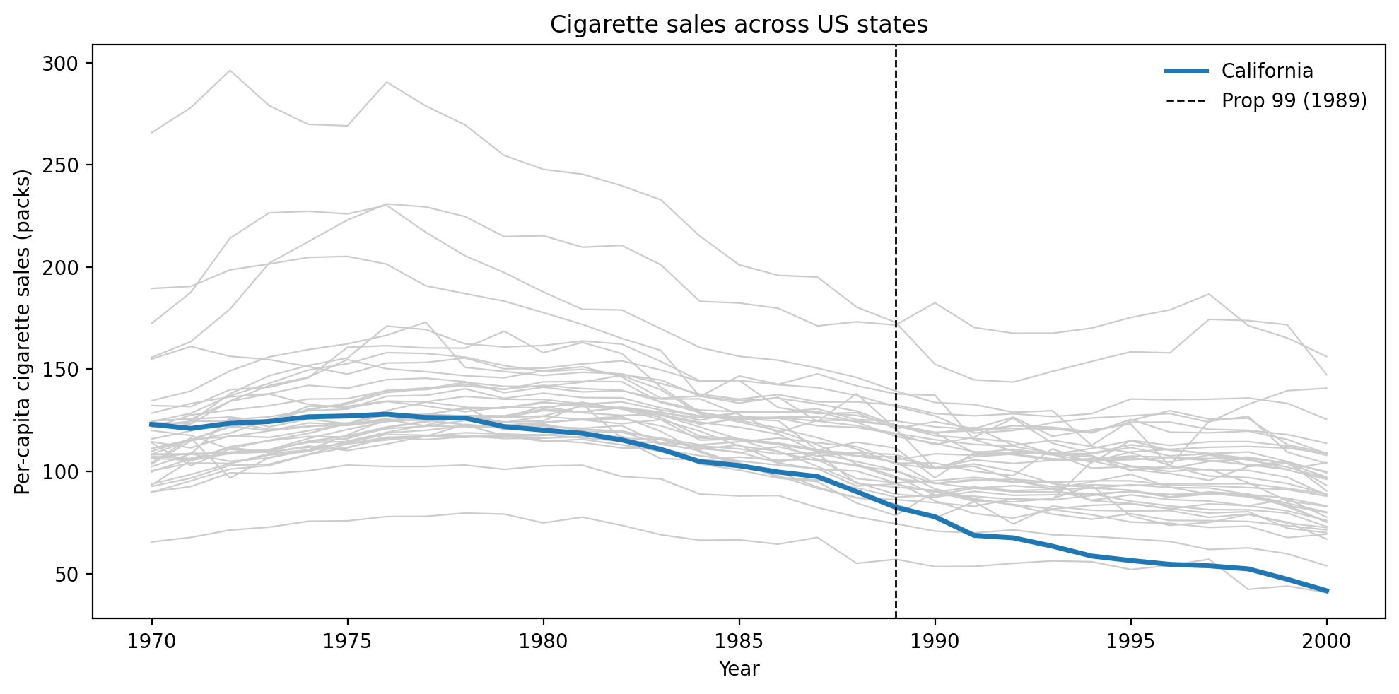
All states share a broad downward trend in cigarette consumption from the 1970s onward, reflecting national public-health campaigns and changing social norms. California (blue) tracks the middle of the donor pack in the pre-period, confirming that a synthetic control constructed from these states is plausible. After Proposition 99 takes effect in 1989, California’s trajectory drops noticeably below the donor band — the gap between the blue line and the grey bundle is the visual signature of the treatment effect we aim to estimate.
Before the experiment: assessing the design#
Will this experiment detect the effect we care about? Before committing budget, we should assess whether the synthetic control design can plausibly recover an effect from the available donor pool. Everything in this section uses only pre-period data — no post-period observations are needed.
We begin with visual checks — inspecting donor correlations and the convex hull condition — then move to quantitative tools: donor pool quality scoring, a dress rehearsal, and a power analysis. For the quantitative tools we fit the SC model on historical data alone using SyntheticControl.from_pre_period().
Donor pool selection#
Before fitting, it is good practice to inspect pairwise correlations among units in the pre-treatment period. The donor pool should consist of units not affected by the intervention and driven by the same structural process as the treated unit [Abadie, 2021]. A poorly chosen pool forces the synthetic control to extrapolate rather than interpolate, introducing bias [Abadie et al., 2010]. Donor units that experienced similar shocks or policy changes during the study period should also be excluded [Abadie et al., 2015].
For the Proposition 99 analysis, Abadie et al. [2010] excluded states that enacted large tobacco tax increases or control programs during the study period. The dataset we use here already reflects their curated 38-state donor pool.
Tip
Beyond correlations, practitioners should verify that (a) no donor units were affected by similar interventions during the study window [Abadie et al., 2015] and (b) relevant pre-treatment covariates are also balanced, when available — careless donor pool composition is one of the most consequential choices in SC analysis, and pre-treatment outcome matching alone may be insufficient [Pickett et al., 2025].
pre = df.loc[:treatment_time]
corr, ax = cp.plot_correlations(
    pre, columns=control_units + [treated_unit], figsize=(16, 14)
)
ax.set(title="Pre-treatment pairwise correlations (1970–1988)");
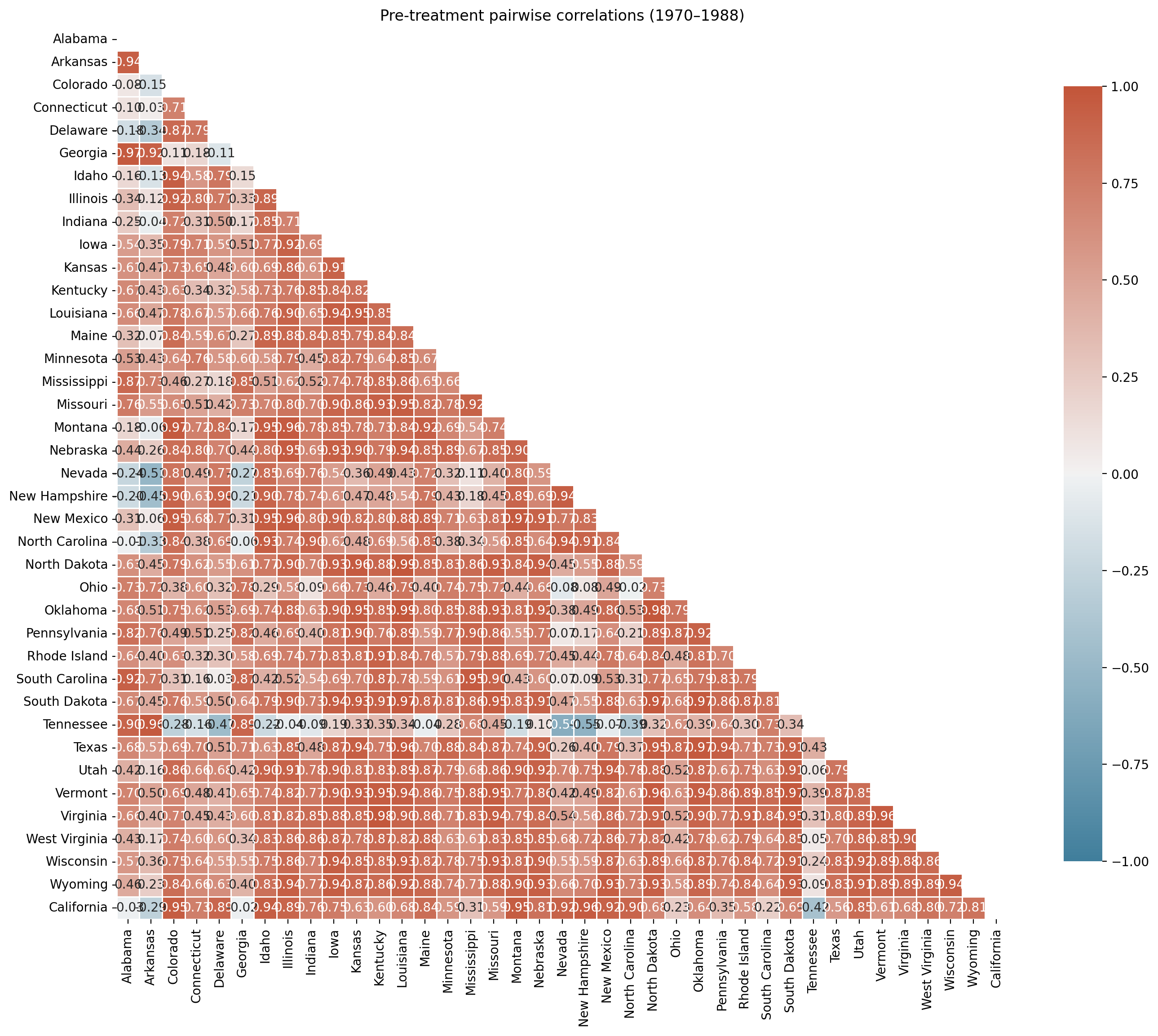
Most control states are positively correlated with California in the pre-period, reflecting shared national trends in declining cigarette consumption. However, a few states show negative or near-zero correlations — these units’ pre-treatment trajectories moved in the opposite direction to California’s and would force the model to assign them negative weight (which the Dirichlet prior prohibits) or effectively ignore them.
Including such units is not harmful in a strict sense — they will receive near-zero weight — but they add noise to the optimisation and can slow convergence. More importantly, Abadie [2021] recommends that the donor pool consist of units “driven by the same structural process” as the treated unit, and a negative pre-treatment correlation is evidence against that assumption.
We apply a correlation threshold of 0.0 to exclude states whose pre-treatment cigarette sales moved in the opposite direction to California’s. This is a conservative choice — it only removes clearly unsuitable donors rather than aggressively pruning the pool. A stricter threshold (e.g., 0.5) would retain only the best-matching states but risks excluding units that contribute useful information. The right threshold depends on domain knowledge and the number of donors available; with 38 candidates, we can afford to be selective without starving the model of donors.
from matplotlib.colors import Normalize

STATE_ABBREV = {
    "Alabama": "AL",
    "Arkansas": "AR",
    "California": "CA",
    "Colorado": "CO",
    "Connecticut": "CT",
    "Delaware": "DE",
    "Georgia": "GA",
    "Idaho": "ID",
    "Illinois": "IL",
    "Indiana": "IN",
    "Iowa": "IA",
    "Kansas": "KS",
    "Kentucky": "KY",
    "Louisiana": "LA",
    "Maine": "ME",
    "Minnesota": "MN",
    "Mississippi": "MS",
    "Missouri": "MO",
    "Montana": "MT",
    "Nebraska": "NE",
    "Nevada": "NV",
    "New Hampshire": "NH",
    "New Mexico": "NM",
    "North Carolina": "NC",
    "North Dakota": "ND",
    "Ohio": "OH",
    "Oklahoma": "OK",
    "Pennsylvania": "PA",
    "Rhode Island": "RI",
    "South Carolina": "SC_state",
    "South Dakota": "SD",
    "Tennessee": "TN",
    "Texas": "TX",
    "Utah": "UT",
    "Vermont": "VT",
    "Virginia": "VA",
    "West Virginia": "WV",
    "Wisconsin": "WI",
    "Wyoming": "WY",
}

# Tile grid positions (col, row) approximating US geography.
GRID = {
    "AK": (0, 0),
    "ME": (10, 0),
    "VT": (8, 1),
    "NH": (9, 1),
    "WA": (0, 2),
    "ID": (1, 2),
    "MT": (2, 2),
    "ND": (3, 2),
    "MN": (4, 2),
    "WI": (5, 2),
    "MI": (7, 2),
    "NY": (8, 2),
    "MA": (9, 2),
    "RI": (10, 2),
    "CT": (11, 2),
    "OR": (0, 3),
    "NV": (1, 3),
    "WY": (2, 3),
    "SD": (3, 3),
    "IA": (4, 3),
    "IL": (5, 3),
    "IN": (6, 3),
    "OH": (7, 3),
    "PA": (8, 3),
    "NJ": (9, 3),
    "CA": (0, 4),
    "UT": (1, 4),
    "CO": (2, 4),
    "NE": (3, 4),
    "MO": (4, 4),
    "KY": (5, 4),
    "WV": (6, 4),
    "VA": (7, 4),
    "MD": (8, 4),
    "DE": (9, 4),
    "AZ": (1, 5),
    "NM": (2, 5),
    "KS": (3, 5),
    "AR": (4, 5),
    "TN": (5, 5),
    "NC": (6, 5),
    "SC": (7, 5),
    "OK": (3, 6),
    "LA": (4, 6),
    "MS": (5, 6),
    "AL": (6, 6),
    "GA": (7, 6),
    "HI": (0, 7),
    "TX": (3, 7),
    "FL": (8, 7),
}

calif_corr = corr[treated_unit].drop(treated_unit)
abbrev_corr = {
    STATE_ABBREV[name]: val for name, val in calif_corr.items() if name in STATE_ABBREV
}
abbrev_corr = {("SC" if k == "SC_state" else k): v for k, v in abbrev_corr.items()}

r = 0.46
spacing = 1.0
cmap = plt.cm.RdYlGn
norm = Normalize(vmin=-0.2, vmax=1.0)

fig, ax = plt.subplots(figsize=(12, 7))
for abbr, (col, row) in GRID.items():
    x = col * spacing
    y = -row * spacing

    if abbr == "CA":
        color, ec = "C0", "C0"
        label = "CA\n(treated)"
    elif abbr in abbrev_corr:
        color = cmap(norm(abbrev_corr[abbr]))
        ec = "0.6"
        label = f"{abbr}\n{abbrev_corr[abbr]:.2f}"
    else:
        color, ec = "0.93", "0.8"
        label = abbr

    circle = plt.Circle((x, y), r, facecolor=color, edgecolor=ec, linewidth=1.2)
    ax.add_patch(circle)
    ax.text(
        x,
        y,
        label,
        ha="center",
        va="center",
        fontsize=6,
        fontweight="bold" if abbr == "CA" else "normal",
        color="white" if abbr == "CA" else "0.15",
    )

sm = plt.cm.ScalarMappable(cmap=cmap, norm=norm)
sm.set_array([])
cbar = fig.colorbar(sm, ax=ax, shrink=0.6, aspect=25, pad=0.02)
cbar.set_label("Correlation with California (pre-treatment)")

ax.set_aspect("equal")
ax.autoscale_view()
ax.axis("off")
ax.set_title(
    "Pre-treatment correlation with California by state",
    fontsize=14,
    fontweight="bold",
    pad=15,
)
fig.tight_layout()
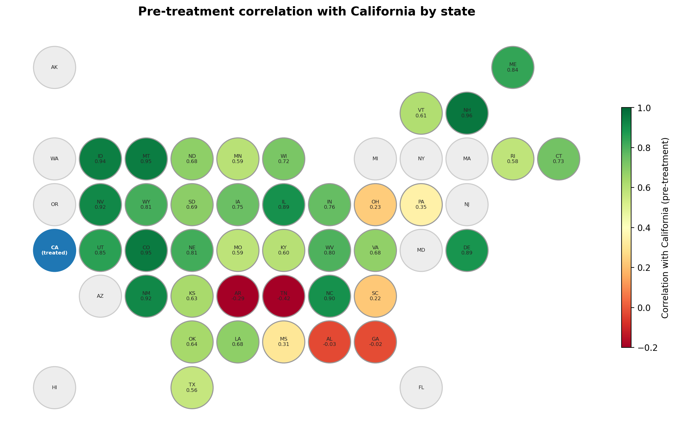
The hex map reveals a clear spatial pattern in donor quality. States in the West and Upper Midwest tend to show the highest correlations with California — they share similar secular trends in cigarette consumption. States in the South and Deep South are weaker donors, and a few show near-zero or negative correlations. Grey hexagons are states excluded from the original Abadie et al. [2010] donor pool (they enacted tobacco legislation during the study period). This spatial view complements the heatmap above by making it easy to spot regional clusters of strong and weak donors.
correlation_threshold = 0.0

calif_corr = corr[treated_unit].drop(treated_unit)
excluded = calif_corr[calif_corr < correlation_threshold].index.tolist()
control_units = [s for s in control_units if s not in excluded]

print(f"Correlation threshold: {correlation_threshold}")
print(f"Excluded {len(excluded)} states: {excluded}")
print(f"Remaining donor pool: {len(control_units)} states")
Correlation threshold: 0.0
Excluded 4 states: ['Alabama', 'Arkansas', 'Georgia', 'Tennessee']
Remaining donor pool: 34 states
The convex hull condition#
The synthetic control method uses non-negative weights that sum to one. This means the synthetic control is a convex combination of the control units — it can only produce values within the range spanned by the controls at each time point [Abadie, 2021]. The convex hull requirement is a direct consequence of the non-negativity and sum-to-one constraints on the weights [Doudchenko and Imbens, 2016].
Note
For the method to work well, the treated unit’s pre-intervention trajectory should lie within the “envelope” of the control units. If all controls are consistently above or below the treated unit, the method cannot construct an accurate counterfactual. Abadie [2021] discusses this condition at length in §4.3.
CausalPy automatically checks this assumption when you create a SyntheticControl object and will issue a warning if violated. The donor_pool_quality() tool in the next section quantifies this condition automatically alongside other diagnostics. See the Convex hull condition glossary entry and Abadie et al. [2010] for more details. The Augmented Synthetic Control Method [Ben-Michael et al., 2021] can handle cases where this assumption is violated.
Create a SyntheticControl design object from the pre-period#
We create a design object using only the pre-intervention data (1970–1988). This object provides the design assessment methods — donor pool quality scoring, dress rehearsal, and power analysis — without requiring post-intervention data.
Note
On the choice of prior for the observation noise. The default WeightedSumFitter likelihood is \(y \sim \mathrm{Normal}(\mu, \sigma)\) with \(\sigma \sim \mathrm{HalfNormal}(1)\). For Proposition 99 the outcome (per-capita cigarette sales) ranges from roughly 40 to 130 packs, so a \(\sigma\) prior centred near 1 is far too tight relative to the data scale. We override it with \(\sigma \sim \mathrm{HalfNormal}(10)\) below. In practice this halves the wall-clock time of the design fit, roughly doubles effective sample size, and silences the overflow encountered in dot warnings that NUTS otherwise emits during warmup adaptation. As a rule of thumb when modelling a new outcome, scale this prior to the order of magnitude of the outcome’s standard deviation.
pre_data = df[df.index < treatment_time]

design = cp.SyntheticControl.from_pre_period(
    pre_data,
    control_units=control_units,
    treated_units=[treated_unit],
    model=cp.pymc_models.WeightedSumFitter(
        priors={
            "y_hat": Prior(
                "Normal",
                sigma=Prior("HalfNormal", sigma=10, dims=["treated_units"]),
                dims=["obs_ind", "treated_units"],
            ),
        },
        sample_kwargs={
            "target_accept": 0.95,
            "random_seed": seed,
        },
    ),
)
Show code cell output
Initializing NUTS using jitter+adapt_diag...
Multiprocess sampling (4 chains in 4 jobs)
NUTS: [beta, y_hat_sigma]
Sampling 4 chains for 1_000 tune and 1_000 draw iterations (4_000 + 4_000 draws total) took 6 seconds.
Sampling: [beta, y_hat, y_hat_sigma]
Sampling: [y_hat]
Sampling: [y_hat]
Sampling: [y_hat]
Is the donor pool adequate?#
Abadie [2021] recommends a structured feasibility assessment before applying the synthetic control method. donor_pool_quality() implements this assessment by aggregating three diagnostics into a scored summary: mean donor correlation, convex hull condition coverage (what fraction of pre-period time points fall within the control envelope), and weight concentration (effective number of donors via the Dirichlet weights). The weight concentration metric is motivated by the observation that SC solutions tend to be sparse — few donors receive non-zero weights — and while some sparsity is natural, extreme concentration in a single donor makes the estimate fragile to that unit’s idiosyncratic shocks [Abadie, 2021]. A pool rated “good” on all three dimensions gives confidence the SC can produce a reliable counterfactual. GeoLift [Meta Incubator, 2022] implements a parallel composite diagnostic in the frequentist setting.
quality = design.donor_pool_quality()
quality.summary()
| metric | value | assessment | |
|---|---|---|---|
| 0 | Mean donor correlation | 0.635 | acceptable |
| 1 | Convex hull coverage | 100.0% | good |
| 2 | Effective number of donors | 19.38 | good |
| 3 | Overall quality | acceptable | acceptable |
What is the minimum detectable effect size?#
The dress rehearsal tests a single effect size. A power analysis extends this across a range of candidates to produce a Bayesian power curve — for each effect size, what fraction of simulations successfully detect the effect? Simulation-based power analysis is the industry standard for SC experiment design, pioneered by GeoLift [Meta Incubator, 2022] and supported by Athey and Imbens [2017], who note the importance of supplementary simulation exercises to strengthen the credibility of identification strategies.
How it works. For each candidate effect size, multiple simulations are run. Each simulation:
Adds random noise (drawn from the fitted model’s residual distribution) to the treated unit in the pre-period, creating a realistic “what if we ran this experiment again?” scenario.
Fits a fresh SC on the noisy pre-period data.
Runs a dress rehearsal with the candidate effect size — injecting the effect into the pseudo-post window as described above.
Evaluates whether the effect was detected: is the posterior probability that the cumulative impact is positive greater than 0.95 (i.e.
P(impact > 0) > 0.95)?
Note the difference from the dress rehearsal criterion: the power analysis asks whether the model can tell that an effect of the expected sign exists, not whether it recovers the exact magnitude (HDI covers truth). The detection rate across simulations gives the power at that effect size. The minimum detectable effect (MDE) is the smallest effect size where the power curve crosses the conventional 80% threshold.
We use the prob_gt_zero criterion here in preference to the default hdi_excludes_zero. The HDI-based criterion is sign-blind — it counts an HDI bounded away from zero as a detection regardless of which side of zero it sits on, which can flag mis-fit artefacts of the wrong sign as “detections” at small injected effects. prob_gt_zero requires the posterior mass to concentrate on the side of zero matching the injected (positive) effect, giving a more interpretable curve.
Unlike frequentist power (which asks “does the p-value fall below 0.05?”), Bayesian power here asks: what fraction of the cumulative-impact posterior lies above zero? This posterior-based approach to detection is a natural advantage of the Bayesian framework: Brodersen et al. [2015] demonstrate how posterior predictive distributions quantify uncertainty in the counterfactual, and Kim et al. [2020] extend this specifically to synthetic control, arguing that the Bayesian framework provides “straightforward statistical inference” while avoiding the restrictive assumptions of frequentist SC inference.
Note
We use n_simulations=25 and lighter MCMC settings to keep runtime reasonable for documentation builds. In practice, more simulations (50–100) produce smoother power curves.
fast_kwargs = {
    "chains": 4,
    "draws": 500,
    "tune": 500,
    "progressbar": False,
    "target_accept": 0.95,
    "random_seed": 42,
}

power_curve = design.power_analysis(
    effect_sizes=np.linspace(0, 0.25, 6),
    n_simulations=25,
    criterion="prob_gt_zero",
    sample_kwargs=fast_kwargs,
    random_seed=42,
)
Show code cell output
Initializing NUTS using jitter+adapt_diag...
Multiprocess sampling (4 chains in 4 jobs)
NUTS: [beta, y_hat_sigma]
Sampling 4 chains for 500 tune and 500 draw iterations (2_000 + 2_000 draws total) took 3 seconds.
Sampling: [beta, y_hat, y_hat_sigma]
Sampling: [y_hat]
Sampling: [y_hat]
Sampling: [y_hat]
/Users/benjamv/git/CausalPy/causalpy/experiments/synthetic_control.py:128: UserWarning: Control units ['Connecticut' (r=-0.003), 'Minnesota' (r=-0.205), 'Mississippi' (r=-0.009), 'Ohio' (r=-0.156), 'Oklahoma' (r=-0.012), 'Pennsylvania' (r=-0.042), 'Texas' (r=-0.076)] have pre-treatment correlation below 0.0 or undefined with treated unit 'California'. Consider excluding them from the donor pool. Use cp.plot_correlations() to inspect. See Abadie (2021) for guidance on donor pool selection.
  self._check_donor_correlations()
Initializing NUTS using jitter+adapt_diag...
Multiprocess sampling (4 chains in 4 jobs)
NUTS: [beta, y_hat_sigma]
Sampling 4 chains for 500 tune and 500 draw iterations (2_000 + 2_000 draws total) took 3 seconds.
Sampling: [beta, y_hat, y_hat_sigma]
Sampling: [y_hat]
Sampling: [y_hat]
Sampling: [y_hat]
Sampling: [y_hat]
Initializing NUTS using jitter+adapt_diag...
Multiprocess sampling (4 chains in 4 jobs)
NUTS: [beta, y_hat_sigma]
Sampling 4 chains for 500 tune and 500 draw iterations (2_000 + 2_000 draws total) took 3 seconds.
Sampling: [beta, y_hat, y_hat_sigma]
Sampling: [y_hat]
Sampling: [y_hat]
Sampling: [y_hat]
/Users/benjamv/git/CausalPy/causalpy/experiments/synthetic_control.py:128: UserWarning: Control units ['Ohio' (r=-0.181), 'Pennsylvania' (r=-0.023), 'Texas' (r=-0.025)] have pre-treatment correlation below 0.0 or undefined with treated unit 'California'. Consider excluding them from the donor pool. Use cp.plot_correlations() to inspect. See Abadie (2021) for guidance on donor pool selection.
  self._check_donor_correlations()
Initializing NUTS using jitter+adapt_diag...
Multiprocess sampling (4 chains in 4 jobs)
NUTS: [beta, y_hat_sigma]
Sampling 4 chains for 500 tune and 500 draw iterations (2_000 + 2_000 draws total) took 3 seconds.
Sampling: [beta, y_hat, y_hat_sigma]
Sampling: [y_hat]
Sampling: [y_hat]
Sampling: [y_hat]
Sampling: [y_hat]
Initializing NUTS using jitter+adapt_diag...
Multiprocess sampling (4 chains in 4 jobs)
NUTS: [beta, y_hat_sigma]
Sampling 4 chains for 500 tune and 500 draw iterations (2_000 + 2_000 draws total) took 3 seconds.
Sampling: [beta, y_hat, y_hat_sigma]
Sampling: [y_hat]
Sampling: [y_hat]
Sampling: [y_hat]
/Users/benjamv/git/CausalPy/causalpy/experiments/synthetic_control.py:128: UserWarning: Control units ['Kansas' (r=-0.092), 'Ohio' (r=-0.181), 'Pennsylvania' (r=-0.080), 'Texas' (r=-0.060)] have pre-treatment correlation below 0.0 or undefined with treated unit 'California'. Consider excluding them from the donor pool. Use cp.plot_correlations() to inspect. See Abadie (2021) for guidance on donor pool selection.
  self._check_donor_correlations()
Initializing NUTS using jitter+adapt_diag...
Multiprocess sampling (4 chains in 4 jobs)
NUTS: [beta, y_hat_sigma]
Sampling 4 chains for 500 tune and 500 draw iterations (2_000 + 2_000 draws total) took 3 seconds.
Sampling: [beta, y_hat, y_hat_sigma]
Sampling: [y_hat]
Sampling: [y_hat]
Sampling: [y_hat]
Sampling: [y_hat]
/Users/benjamv/git/CausalPy/causalpy/experiments/synthetic_control.py:128: UserWarning: Control units ['Ohio' (r=-0.001)] have pre-treatment correlation below 0.0 or undefined with treated unit 'California'. Consider excluding them from the donor pool. Use cp.plot_correlations() to inspect. See Abadie (2021) for guidance on donor pool selection.
  self._check_donor_correlations()
Initializing NUTS using jitter+adapt_diag...
Multiprocess sampling (4 chains in 4 jobs)
NUTS: [beta, y_hat_sigma]
Sampling 4 chains for 500 tune and 500 draw iterations (2_000 + 2_000 draws total) took 3 seconds.
Sampling: [beta, y_hat, y_hat_sigma]
Sampling: [y_hat]
Sampling: [y_hat]
Sampling: [y_hat]
/Users/benjamv/git/CausalPy/causalpy/experiments/synthetic_control.py:128: UserWarning: Control units ['Kansas' (r=-0.015), 'Minnesota' (r=-0.087), 'Mississippi' (r=-0.165), 'Ohio' (r=-0.250), 'Oklahoma' (r=-0.063), 'Pennsylvania' (r=-0.165), 'South Carolina' (r=-0.027), 'Texas' (r=-0.154)] have pre-treatment correlation below 0.0 or undefined with treated unit 'California'. Consider excluding them from the donor pool. Use cp.plot_correlations() to inspect. See Abadie (2021) for guidance on donor pool selection.
  self._check_donor_correlations()
Initializing NUTS using jitter+adapt_diag...
Multiprocess sampling (4 chains in 4 jobs)
NUTS: [beta, y_hat_sigma]
Sampling 4 chains for 500 tune and 500 draw iterations (2_000 + 2_000 draws total) took 3 seconds.
Sampling: [beta, y_hat, y_hat_sigma]
Sampling: [y_hat]
Sampling: [y_hat]
Sampling: [y_hat]
Sampling: [y_hat]
Initializing NUTS using jitter+adapt_diag...
Multiprocess sampling (4 chains in 4 jobs)
NUTS: [beta, y_hat_sigma]
Sampling 4 chains for 500 tune and 500 draw iterations (2_000 + 2_000 draws total) took 3 seconds.
Sampling: [beta, y_hat, y_hat_sigma]
Sampling: [y_hat]
Sampling: [y_hat]
Sampling: [y_hat]
/Users/benjamv/git/CausalPy/causalpy/experiments/synthetic_control.py:128: UserWarning: Control units ['Connecticut' (r=-0.163), 'Kansas' (r=-0.274), 'Louisiana' (r=-0.107), 'Minnesota' (r=-0.228), 'Mississippi' (r=-0.146), 'North Dakota' (r=-0.110), 'Ohio' (r=-0.463), 'Oklahoma' (r=-0.155), 'Pennsylvania' (r=-0.334), 'South Carolina' (r=-0.071), 'Texas' (r=-0.330)] have pre-treatment correlation below 0.0 or undefined with treated unit 'California'. Consider excluding them from the donor pool. Use cp.plot_correlations() to inspect. See Abadie (2021) for guidance on donor pool selection.
  self._check_donor_correlations()
Initializing NUTS using jitter+adapt_diag...
Multiprocess sampling (4 chains in 4 jobs)
NUTS: [beta, y_hat_sigma]
Sampling 4 chains for 500 tune and 500 draw iterations (2_000 + 2_000 draws total) took 3 seconds.
Sampling: [beta, y_hat, y_hat_sigma]
Sampling: [y_hat]
Sampling: [y_hat]
Sampling: [y_hat]
Sampling: [y_hat]
Initializing NUTS using jitter+adapt_diag...
Multiprocess sampling (4 chains in 4 jobs)
NUTS: [beta, y_hat_sigma]
Sampling 4 chains for 500 tune and 500 draw iterations (2_000 + 2_000 draws total) took 3 seconds.
Sampling: [beta, y_hat, y_hat_sigma]
Sampling: [y_hat]
Sampling: [y_hat]
Sampling: [y_hat]
/Users/benjamv/git/CausalPy/causalpy/experiments/synthetic_control.py:128: UserWarning: Control units ['Connecticut' (r=-0.107), 'Ohio' (r=-0.211)] have pre-treatment correlation below 0.0 or undefined with treated unit 'California'. Consider excluding them from the donor pool. Use cp.plot_correlations() to inspect. See Abadie (2021) for guidance on donor pool selection.
  self._check_donor_correlations()
Initializing NUTS using jitter+adapt_diag...
Multiprocess sampling (4 chains in 4 jobs)
NUTS: [beta, y_hat_sigma]
Sampling 4 chains for 500 tune and 500 draw iterations (2_000 + 2_000 draws total) took 3 seconds.
Sampling: [beta, y_hat, y_hat_sigma]
Sampling: [y_hat]
Sampling: [y_hat]
Sampling: [y_hat]
Sampling: [y_hat]
Initializing NUTS using jitter+adapt_diag...
Multiprocess sampling (4 chains in 4 jobs)
NUTS: [beta, y_hat_sigma]
Sampling 4 chains for 500 tune and 500 draw iterations (2_000 + 2_000 draws total) took 3 seconds.
Sampling: [beta, y_hat, y_hat_sigma]
Sampling: [y_hat]
Sampling: [y_hat]
Sampling: [y_hat]
/Users/benjamv/git/CausalPy/causalpy/experiments/synthetic_control.py:128: UserWarning: Control units ['Kansas' (r=-0.004), 'Ohio' (r=-0.137), 'Pennsylvania' (r=-0.069), 'Texas' (r=-0.023)] have pre-treatment correlation below 0.0 or undefined with treated unit 'California'. Consider excluding them from the donor pool. Use cp.plot_correlations() to inspect. See Abadie (2021) for guidance on donor pool selection.
  self._check_donor_correlations()
Initializing NUTS using jitter+adapt_diag...
Multiprocess sampling (4 chains in 4 jobs)
NUTS: [beta, y_hat_sigma]
Sampling 4 chains for 500 tune and 500 draw iterations (2_000 + 2_000 draws total) took 3 seconds.
Sampling: [beta, y_hat, y_hat_sigma]
Sampling: [y_hat]
Sampling: [y_hat]
Sampling: [y_hat]
Sampling: [y_hat]
/Users/benjamv/git/CausalPy/causalpy/experiments/synthetic_control.py:128: UserWarning: Control units ['Ohio' (r=-0.145)] have pre-treatment correlation below 0.0 or undefined with treated unit 'California'. Consider excluding them from the donor pool. Use cp.plot_correlations() to inspect. See Abadie (2021) for guidance on donor pool selection.
  self._check_donor_correlations()
Initializing NUTS using jitter+adapt_diag...
Multiprocess sampling (4 chains in 4 jobs)
NUTS: [beta, y_hat_sigma]
Sampling 4 chains for 500 tune and 500 draw iterations (2_000 + 2_000 draws total) took 3 seconds.
Sampling: [beta, y_hat, y_hat_sigma]
Sampling: [y_hat]
Sampling: [y_hat]
Sampling: [y_hat]
/Users/benjamv/git/CausalPy/causalpy/experiments/synthetic_control.py:128: UserWarning: Control units ['Connecticut' (r=-0.280), 'Minnesota' (r=-0.069), 'Mississippi' (r=-0.031), 'Ohio' (r=-0.499), 'Oklahoma' (r=-0.005), 'Pennsylvania' (r=-0.165), 'Texas' (r=-0.179)] have pre-treatment correlation below 0.0 or undefined with treated unit 'California'. Consider excluding them from the donor pool. Use cp.plot_correlations() to inspect. See Abadie (2021) for guidance on donor pool selection.
  self._check_donor_correlations()
Initializing NUTS using jitter+adapt_diag...
Multiprocess sampling (4 chains in 4 jobs)
NUTS: [beta, y_hat_sigma]
Sampling 4 chains for 500 tune and 500 draw iterations (2_000 + 2_000 draws total) took 3 seconds.
Sampling: [beta, y_hat, y_hat_sigma]
Sampling: [y_hat]
Sampling: [y_hat]
Sampling: [y_hat]
Sampling: [y_hat]
Initializing NUTS using jitter+adapt_diag...
Multiprocess sampling (4 chains in 4 jobs)
NUTS: [beta, y_hat_sigma]
Sampling 4 chains for 500 tune and 500 draw iterations (2_000 + 2_000 draws total) took 3 seconds.
Sampling: [beta, y_hat, y_hat_sigma]
Sampling: [y_hat]
Sampling: [y_hat]
Sampling: [y_hat]
/Users/benjamv/git/CausalPy/causalpy/experiments/synthetic_control.py:128: UserWarning: Control units ['Connecticut' (r=-0.417), 'Kansas' (r=-0.112), 'Minnesota' (r=-0.118), 'Ohio' (r=-0.313), 'Pennsylvania' (r=-0.194), 'Texas' (r=-0.150)] have pre-treatment correlation below 0.0 or undefined with treated unit 'California'. Consider excluding them from the donor pool. Use cp.plot_correlations() to inspect. See Abadie (2021) for guidance on donor pool selection.
  self._check_donor_correlations()
Initializing NUTS using jitter+adapt_diag...
Multiprocess sampling (4 chains in 4 jobs)
NUTS: [beta, y_hat_sigma]
Sampling 4 chains for 500 tune and 500 draw iterations (2_000 + 2_000 draws total) took 3 seconds.
Sampling: [beta, y_hat, y_hat_sigma]
Sampling: [y_hat]
Sampling: [y_hat]
Sampling: [y_hat]
Sampling: [y_hat]
Initializing NUTS using jitter+adapt_diag...
Multiprocess sampling (4 chains in 4 jobs)
NUTS: [beta, y_hat_sigma]
Sampling 4 chains for 500 tune and 500 draw iterations (2_000 + 2_000 draws total) took 3 seconds.
Sampling: [beta, y_hat, y_hat_sigma]
Sampling: [y_hat]
Sampling: [y_hat]
Sampling: [y_hat]
/Users/benjamv/git/CausalPy/causalpy/experiments/synthetic_control.py:128: UserWarning: Control units ['Delaware' (r=-0.090), 'Ohio' (r=-0.184)] have pre-treatment correlation below 0.0 or undefined with treated unit 'California'. Consider excluding them from the donor pool. Use cp.plot_correlations() to inspect. See Abadie (2021) for guidance on donor pool selection.
  self._check_donor_correlations()
Initializing NUTS using jitter+adapt_diag...
Multiprocess sampling (4 chains in 4 jobs)
NUTS: [beta, y_hat_sigma]
Sampling 4 chains for 500 tune and 500 draw iterations (2_000 + 2_000 draws total) took 3 seconds.
Sampling: [beta, y_hat, y_hat_sigma]
Sampling: [y_hat]
Sampling: [y_hat]
Sampling: [y_hat]
Sampling: [y_hat]
Initializing NUTS using jitter+adapt_diag...
Multiprocess sampling (4 chains in 4 jobs)
NUTS: [beta, y_hat_sigma]
Sampling 4 chains for 500 tune and 500 draw iterations (2_000 + 2_000 draws total) took 3 seconds.
Sampling: [beta, y_hat, y_hat_sigma]
Sampling: [y_hat]
Sampling: [y_hat]
Sampling: [y_hat]
/Users/benjamv/git/CausalPy/causalpy/experiments/synthetic_control.py:128: UserWarning: Control units ['Kansas' (r=-0.054), 'Louisiana' (r=-0.001), 'Minnesota' (r=-0.030), 'Mississippi' (r=-0.172), 'North Dakota' (r=-0.003), 'Ohio' (r=-0.253), 'Oklahoma' (r=-0.100), 'Pennsylvania' (r=-0.121), 'South Carolina' (r=-0.083), 'Texas' (r=-0.137)] have pre-treatment correlation below 0.0 or undefined with treated unit 'California'. Consider excluding them from the donor pool. Use cp.plot_correlations() to inspect. See Abadie (2021) for guidance on donor pool selection.
  self._check_donor_correlations()
Initializing NUTS using jitter+adapt_diag...
Multiprocess sampling (4 chains in 4 jobs)
NUTS: [beta, y_hat_sigma]
Sampling 4 chains for 500 tune and 500 draw iterations (2_000 + 2_000 draws total) took 3 seconds.
Sampling: [beta, y_hat, y_hat_sigma]
Sampling: [y_hat]
Sampling: [y_hat]
Sampling: [y_hat]
Sampling: [y_hat]
/Users/benjamv/git/CausalPy/causalpy/experiments/synthetic_control.py:128: UserWarning: Control units ['Ohio' (r=-0.035)] have pre-treatment correlation below 0.0 or undefined with treated unit 'California'. Consider excluding them from the donor pool. Use cp.plot_correlations() to inspect. See Abadie (2021) for guidance on donor pool selection.
  self._check_donor_correlations()
Initializing NUTS using jitter+adapt_diag...
Multiprocess sampling (4 chains in 4 jobs)
NUTS: [beta, y_hat_sigma]
Sampling 4 chains for 500 tune and 500 draw iterations (2_000 + 2_000 draws total) took 3 seconds.
Sampling: [beta, y_hat, y_hat_sigma]
Sampling: [y_hat]
Sampling: [y_hat]
Sampling: [y_hat]
/Users/benjamv/git/CausalPy/causalpy/experiments/synthetic_control.py:128: UserWarning: Control units ['Kansas' (r=-0.025), 'Ohio' (r=-0.237), 'Pennsylvania' (r=-0.077), 'Texas' (r=-0.044)] have pre-treatment correlation below 0.0 or undefined with treated unit 'California'. Consider excluding them from the donor pool. Use cp.plot_correlations() to inspect. See Abadie (2021) for guidance on donor pool selection.
  self._check_donor_correlations()
Initializing NUTS using jitter+adapt_diag...
Multiprocess sampling (4 chains in 4 jobs)
NUTS: [beta, y_hat_sigma]
Sampling 4 chains for 500 tune and 500 draw iterations (2_000 + 2_000 draws total) took 3 seconds.
Sampling: [beta, y_hat, y_hat_sigma]
Sampling: [y_hat]
Sampling: [y_hat]
Sampling: [y_hat]
Sampling: [y_hat]
/Users/benjamv/git/CausalPy/causalpy/experiments/synthetic_control.py:128: UserWarning: Control units ['Ohio' (r=-0.073)] have pre-treatment correlation below 0.0 or undefined with treated unit 'California'. Consider excluding them from the donor pool. Use cp.plot_correlations() to inspect. See Abadie (2021) for guidance on donor pool selection.
  self._check_donor_correlations()
Initializing NUTS using jitter+adapt_diag...
Multiprocess sampling (4 chains in 4 jobs)
NUTS: [beta, y_hat_sigma]
Sampling 4 chains for 500 tune and 500 draw iterations (2_000 + 2_000 draws total) took 3 seconds.
Sampling: [beta, y_hat, y_hat_sigma]
Sampling: [y_hat]
Sampling: [y_hat]
Sampling: [y_hat]
/Users/benjamv/git/CausalPy/causalpy/experiments/synthetic_control.py:128: UserWarning: Control units ['Connecticut' (r=-0.140), 'Kansas' (r=-0.116), 'Louisiana' (r=-0.039), 'Minnesota' (r=-0.022), 'Mississippi' (r=-0.109), 'Ohio' (r=-0.469), 'Oklahoma' (r=-0.072), 'Pennsylvania' (r=-0.209), 'Texas' (r=-0.224)] have pre-treatment correlation below 0.0 or undefined with treated unit 'California'. Consider excluding them from the donor pool. Use cp.plot_correlations() to inspect. See Abadie (2021) for guidance on donor pool selection.
  self._check_donor_correlations()
Initializing NUTS using jitter+adapt_diag...
Multiprocess sampling (4 chains in 4 jobs)
NUTS: [beta, y_hat_sigma]
Sampling 4 chains for 500 tune and 500 draw iterations (2_000 + 2_000 draws total) took 3 seconds.
Sampling: [beta, y_hat, y_hat_sigma]
Sampling: [y_hat]
Sampling: [y_hat]
Sampling: [y_hat]
Sampling: [y_hat]
/Users/benjamv/git/CausalPy/causalpy/experiments/synthetic_control.py:128: UserWarning: Control units ['Mississippi' (r=-0.074), 'Ohio' (r=-0.164), 'Pennsylvania' (r=-0.033), 'South Carolina' (r=-0.089)] have pre-treatment correlation below 0.0 or undefined with treated unit 'California'. Consider excluding them from the donor pool. Use cp.plot_correlations() to inspect. See Abadie (2021) for guidance on donor pool selection.
  self._check_donor_correlations()
Initializing NUTS using jitter+adapt_diag...
Multiprocess sampling (4 chains in 4 jobs)
NUTS: [beta, y_hat_sigma]
Sampling 4 chains for 500 tune and 500 draw iterations (2_000 + 2_000 draws total) took 3 seconds.
Sampling: [beta, y_hat, y_hat_sigma]
Sampling: [y_hat]
Sampling: [y_hat]
Sampling: [y_hat]
/Users/benjamv/git/CausalPy/causalpy/experiments/synthetic_control.py:128: UserWarning: Control units ['Kansas' (r=-0.437), 'Kentucky' (r=-0.059), 'Louisiana' (r=-0.333), 'Maine' (r=-0.002), 'Minnesota' (r=-0.032), 'Mississippi' (r=-0.457), 'Missouri' (r=-0.190), 'North Dakota' (r=-0.358), 'Ohio' (r=-0.493), 'Oklahoma' (r=-0.401), 'Pennsylvania' (r=-0.468), 'Rhode Island' (r=-0.102), 'South Carolina' (r=-0.309), 'South Dakota' (r=-0.216), 'Texas' (r=-0.443), 'Vermont' (r=-0.283), 'Virginia' (r=-0.060)] have pre-treatment correlation below 0.0 or undefined with treated unit 'California'. Consider excluding them from the donor pool. Use cp.plot_correlations() to inspect. See Abadie (2021) for guidance on donor pool selection.
  self._check_donor_correlations()
Initializing NUTS using jitter+adapt_diag...
Multiprocess sampling (4 chains in 4 jobs)
NUTS: [beta, y_hat_sigma]
Sampling 4 chains for 500 tune and 500 draw iterations (2_000 + 2_000 draws total) took 3 seconds.
Sampling: [beta, y_hat, y_hat_sigma]
Sampling: [y_hat]
Sampling: [y_hat]
Sampling: [y_hat]
Sampling: [y_hat]
Initializing NUTS using jitter+adapt_diag...
Multiprocess sampling (4 chains in 4 jobs)
NUTS: [beta, y_hat_sigma]
Sampling 4 chains for 500 tune and 500 draw iterations (2_000 + 2_000 draws total) took 3 seconds.
Sampling: [beta, y_hat, y_hat_sigma]
Sampling: [y_hat]
Sampling: [y_hat]
Sampling: [y_hat]
/Users/benjamv/git/CausalPy/causalpy/experiments/synthetic_control.py:128: UserWarning: Control units ['Kansas' (r=-0.037), 'Mississippi' (r=-0.038), 'Ohio' (r=-0.250), 'Pennsylvania' (r=-0.146), 'Texas' (r=-0.095)] have pre-treatment correlation below 0.0 or undefined with treated unit 'California'. Consider excluding them from the donor pool. Use cp.plot_correlations() to inspect. See Abadie (2021) for guidance on donor pool selection.
  self._check_donor_correlations()
Initializing NUTS using jitter+adapt_diag...
Multiprocess sampling (4 chains in 4 jobs)
NUTS: [beta, y_hat_sigma]
Sampling 4 chains for 500 tune and 500 draw iterations (2_000 + 2_000 draws total) took 3 seconds.
Sampling: [beta, y_hat, y_hat_sigma]
Sampling: [y_hat]
Sampling: [y_hat]
Sampling: [y_hat]
Sampling: [y_hat]
/Users/benjamv/git/CausalPy/causalpy/experiments/synthetic_control.py:128: UserWarning: Control units ['Ohio' (r=-0.059)] have pre-treatment correlation below 0.0 or undefined with treated unit 'California'. Consider excluding them from the donor pool. Use cp.plot_correlations() to inspect. See Abadie (2021) for guidance on donor pool selection.
  self._check_donor_correlations()
Initializing NUTS using jitter+adapt_diag...
Multiprocess sampling (4 chains in 4 jobs)
NUTS: [beta, y_hat_sigma]
Sampling 4 chains for 500 tune and 500 draw iterations (2_000 + 2_000 draws total) took 3 seconds.
Sampling: [beta, y_hat, y_hat_sigma]
Sampling: [y_hat]
Sampling: [y_hat]
Sampling: [y_hat]
/Users/benjamv/git/CausalPy/causalpy/experiments/synthetic_control.py:128: UserWarning: Control units ['Connecticut' (r=-0.026), 'Kansas' (r=-0.179), 'Louisiana' (r=-0.030), 'Minnesota' (r=-0.071), 'Mississippi' (r=-0.139), 'North Dakota' (r=-0.044), 'Ohio' (r=-0.419), 'Oklahoma' (r=-0.152), 'Pennsylvania' (r=-0.315), 'South Carolina' (r=-0.025), 'Texas' (r=-0.269)] have pre-treatment correlation below 0.0 or undefined with treated unit 'California'. Consider excluding them from the donor pool. Use cp.plot_correlations() to inspect. See Abadie (2021) for guidance on donor pool selection.
  self._check_donor_correlations()
Initializing NUTS using jitter+adapt_diag...
Multiprocess sampling (4 chains in 4 jobs)
NUTS: [beta, y_hat_sigma]
Sampling 4 chains for 500 tune and 500 draw iterations (2_000 + 2_000 draws total) took 3 seconds.
Sampling: [beta, y_hat, y_hat_sigma]
Sampling: [y_hat]
Sampling: [y_hat]
Sampling: [y_hat]
Sampling: [y_hat]
/Users/benjamv/git/CausalPy/causalpy/experiments/synthetic_control.py:128: UserWarning: Control units ['Ohio' (r=-0.039)] have pre-treatment correlation below 0.0 or undefined with treated unit 'California'. Consider excluding them from the donor pool. Use cp.plot_correlations() to inspect. See Abadie (2021) for guidance on donor pool selection.
  self._check_donor_correlations()
Initializing NUTS using jitter+adapt_diag...
Multiprocess sampling (4 chains in 4 jobs)
NUTS: [beta, y_hat_sigma]
Sampling 4 chains for 500 tune and 500 draw iterations (2_000 + 2_000 draws total) took 3 seconds.
Sampling: [beta, y_hat, y_hat_sigma]
Sampling: [y_hat]
Sampling: [y_hat]
Sampling: [y_hat]
/Users/benjamv/git/CausalPy/causalpy/experiments/synthetic_control.py:128: UserWarning: Control units ['Connecticut' (r=-0.175), 'Minnesota' (r=-0.004), 'Ohio' (r=-0.357), 'Pennsylvania' (r=-0.098), 'Texas' (r=-0.098)] have pre-treatment correlation below 0.0 or undefined with treated unit 'California'. Consider excluding them from the donor pool. Use cp.plot_correlations() to inspect. See Abadie (2021) for guidance on donor pool selection.
  self._check_donor_correlations()
Initializing NUTS using jitter+adapt_diag...
Multiprocess sampling (4 chains in 4 jobs)
NUTS: [beta, y_hat_sigma]
Sampling 4 chains for 500 tune and 500 draw iterations (2_000 + 2_000 draws total) took 3 seconds.
Sampling: [beta, y_hat, y_hat_sigma]
Sampling: [y_hat]
Sampling: [y_hat]
Sampling: [y_hat]
Sampling: [y_hat]
/Users/benjamv/git/CausalPy/causalpy/experiments/synthetic_control.py:128: UserWarning: Control units ['Ohio' (r=-0.023), 'South Carolina' (r=-0.014)] have pre-treatment correlation below 0.0 or undefined with treated unit 'California'. Consider excluding them from the donor pool. Use cp.plot_correlations() to inspect. See Abadie (2021) for guidance on donor pool selection.
  self._check_donor_correlations()
Initializing NUTS using jitter+adapt_diag...
Multiprocess sampling (4 chains in 4 jobs)
NUTS: [beta, y_hat_sigma]
Sampling 4 chains for 500 tune and 500 draw iterations (2_000 + 2_000 draws total) took 3 seconds.
Sampling: [beta, y_hat, y_hat_sigma]
Sampling: [y_hat]
Sampling: [y_hat]
Sampling: [y_hat]
/Users/benjamv/git/CausalPy/causalpy/experiments/synthetic_control.py:128: UserWarning: Control units ['Kansas' (r=-0.391), 'Kentucky' (r=-0.032), 'Louisiana' (r=-0.237), 'Minnesota' (r=-0.112), 'Mississippi' (r=-0.364), 'Missouri' (r=-0.093), 'North Dakota' (r=-0.304), 'Ohio' (r=-0.385), 'Oklahoma' (r=-0.323), 'Pennsylvania' (r=-0.423), 'Rhode Island' (r=-0.132), 'South Carolina' (r=-0.229), 'South Dakota' (r=-0.152), 'Texas' (r=-0.388), 'Vermont' (r=-0.158)] have pre-treatment correlation below 0.0 or undefined with treated unit 'California'. Consider excluding them from the donor pool. Use cp.plot_correlations() to inspect. See Abadie (2021) for guidance on donor pool selection.
  self._check_donor_correlations()
Initializing NUTS using jitter+adapt_diag...
Multiprocess sampling (4 chains in 4 jobs)
NUTS: [beta, y_hat_sigma]
Sampling 4 chains for 500 tune and 500 draw iterations (2_000 + 2_000 draws total) took 3 seconds.
Sampling: [beta, y_hat, y_hat_sigma]
Sampling: [y_hat]
Sampling: [y_hat]
Sampling: [y_hat]
Sampling: [y_hat]
Initializing NUTS using jitter+adapt_diag...
Multiprocess sampling (4 chains in 4 jobs)
NUTS: [beta, y_hat_sigma]
Sampling 4 chains for 500 tune and 500 draw iterations (2_000 + 2_000 draws total) took 3 seconds.
Sampling: [beta, y_hat, y_hat_sigma]
Sampling: [y_hat]
Sampling: [y_hat]
Sampling: [y_hat]
/Users/benjamv/git/CausalPy/causalpy/experiments/synthetic_control.py:128: UserWarning: Control units ['Kansas' (r=-0.043), 'Minnesota' (r=-0.026), 'Mississippi' (r=-0.038), 'Ohio' (r=-0.040), 'Pennsylvania' (r=-0.088), 'Texas' (r=-0.043)] have pre-treatment correlation below 0.0 or undefined with treated unit 'California'. Consider excluding them from the donor pool. Use cp.plot_correlations() to inspect. See Abadie (2021) for guidance on donor pool selection.
  self._check_donor_correlations()
Initializing NUTS using jitter+adapt_diag...
Multiprocess sampling (4 chains in 4 jobs)
NUTS: [beta, y_hat_sigma]
Sampling 4 chains for 500 tune and 500 draw iterations (2_000 + 2_000 draws total) took 3 seconds.
Sampling: [beta, y_hat, y_hat_sigma]
Sampling: [y_hat]
Sampling: [y_hat]
Sampling: [y_hat]
Sampling: [y_hat]
Initializing NUTS using jitter+adapt_diag...
Multiprocess sampling (4 chains in 4 jobs)
NUTS: [beta, y_hat_sigma]
Sampling 4 chains for 500 tune and 500 draw iterations (2_000 + 2_000 draws total) took 3 seconds.
Sampling: [beta, y_hat, y_hat_sigma]
Sampling: [y_hat]
Sampling: [y_hat]
Sampling: [y_hat]
/Users/benjamv/git/CausalPy/causalpy/experiments/synthetic_control.py:128: UserWarning: Control units ['Kansas' (r=-0.087), 'Mississippi' (r=-0.021), 'North Dakota' (r=-0.032), 'Ohio' (r=-0.139), 'Oklahoma' (r=-0.016), 'Pennsylvania' (r=-0.098), 'Texas' (r=-0.044)] have pre-treatment correlation below 0.0 or undefined with treated unit 'California'. Consider excluding them from the donor pool. Use cp.plot_correlations() to inspect. See Abadie (2021) for guidance on donor pool selection.
  self._check_donor_correlations()
Initializing NUTS using jitter+adapt_diag...
Multiprocess sampling (4 chains in 4 jobs)
NUTS: [beta, y_hat_sigma]
Sampling 4 chains for 500 tune and 500 draw iterations (2_000 + 2_000 draws total) took 3 seconds.
Sampling: [beta, y_hat, y_hat_sigma]
Sampling: [y_hat]
Sampling: [y_hat]
Sampling: [y_hat]
Sampling: [y_hat]
/Users/benjamv/git/CausalPy/causalpy/experiments/synthetic_control.py:128: UserWarning: Control units ['Ohio' (r=-0.028)] have pre-treatment correlation below 0.0 or undefined with treated unit 'California'. Consider excluding them from the donor pool. Use cp.plot_correlations() to inspect. See Abadie (2021) for guidance on donor pool selection.
  self._check_donor_correlations()
Initializing NUTS using jitter+adapt_diag...
Multiprocess sampling (4 chains in 4 jobs)
NUTS: [beta, y_hat_sigma]
Sampling 4 chains for 500 tune and 500 draw iterations (2_000 + 2_000 draws total) took 3 seconds.
Sampling: [beta, y_hat, y_hat_sigma]
Sampling: [y_hat]
Sampling: [y_hat]
Sampling: [y_hat]
/Users/benjamv/git/CausalPy/causalpy/experiments/synthetic_control.py:128: UserWarning: Control units ['Kansas' (r=-0.162), 'Louisiana' (r=-0.123), 'Mississippi' (r=-0.277), 'Missouri' (r=-0.036), 'North Dakota' (r=-0.092), 'Ohio' (r=-0.360), 'Oklahoma' (r=-0.165), 'Pennsylvania' (r=-0.259), 'Rhode Island' (r=-0.040), 'South Carolina' (r=-0.096), 'South Dakota' (r=-0.030), 'Texas' (r=-0.233)] have pre-treatment correlation below 0.0 or undefined with treated unit 'California'. Consider excluding them from the donor pool. Use cp.plot_correlations() to inspect. See Abadie (2021) for guidance on donor pool selection.
  self._check_donor_correlations()
Initializing NUTS using jitter+adapt_diag...
Multiprocess sampling (4 chains in 4 jobs)
NUTS: [beta, y_hat_sigma]
Sampling 4 chains for 500 tune and 500 draw iterations (2_000 + 2_000 draws total) took 3 seconds.
Sampling: [beta, y_hat, y_hat_sigma]
Sampling: [y_hat]
Sampling: [y_hat]
Sampling: [y_hat]
Sampling: [y_hat]
/Users/benjamv/git/CausalPy/causalpy/experiments/synthetic_control.py:128: UserWarning: Control units ['Ohio' (r=-0.331), 'Pennsylvania' (r=-0.093)] have pre-treatment correlation below 0.0 or undefined with treated unit 'California'. Consider excluding them from the donor pool. Use cp.plot_correlations() to inspect. See Abadie (2021) for guidance on donor pool selection.
  self._check_donor_correlations()
Initializing NUTS using jitter+adapt_diag...
Multiprocess sampling (4 chains in 4 jobs)
NUTS: [beta, y_hat_sigma]
Sampling 4 chains for 500 tune and 500 draw iterations (2_000 + 2_000 draws total) took 3 seconds.
Sampling: [beta, y_hat, y_hat_sigma]
Sampling: [y_hat]
Sampling: [y_hat]
Sampling: [y_hat]
/Users/benjamv/git/CausalPy/causalpy/experiments/synthetic_control.py:128: UserWarning: Control units ['Connecticut' (r=-0.295), 'Iowa' (r=-0.013), 'Kansas' (r=-0.352), 'Louisiana' (r=-0.247), 'Minnesota' (r=-0.330), 'Mississippi' (r=-0.256), 'Missouri' (r=-0.077), 'Nebraska' (r=-0.117), 'North Dakota' (r=-0.241), 'Ohio' (r=-0.662), 'Oklahoma' (r=-0.307), 'Pennsylvania' (r=-0.475), 'South Carolina' (r=-0.105), 'South Dakota' (r=-0.071), 'Texas' (r=-0.501), 'Vermont' (r=-0.053), 'Wisconsin' (r=-0.000)] have pre-treatment correlation below 0.0 or undefined with treated unit 'California'. Consider excluding them from the donor pool. Use cp.plot_correlations() to inspect. See Abadie (2021) for guidance on donor pool selection.
  self._check_donor_correlations()
Initializing NUTS using jitter+adapt_diag...
Multiprocess sampling (4 chains in 4 jobs)
NUTS: [beta, y_hat_sigma]
Sampling 4 chains for 500 tune and 500 draw iterations (2_000 + 2_000 draws total) took 2 seconds.
Sampling: [beta, y_hat, y_hat_sigma]
Sampling: [y_hat]
Sampling: [y_hat]
Sampling: [y_hat]
Sampling: [y_hat]
Initializing NUTS using jitter+adapt_diag...
Multiprocess sampling (4 chains in 4 jobs)
NUTS: [beta, y_hat_sigma]
Sampling 4 chains for 500 tune and 500 draw iterations (2_000 + 2_000 draws total) took 3 seconds.
Sampling: [beta, y_hat, y_hat_sigma]
Sampling: [y_hat]
Sampling: [y_hat]
Sampling: [y_hat]
/Users/benjamv/git/CausalPy/causalpy/experiments/synthetic_control.py:128: UserWarning: Control units ['Kansas' (r=-0.280), 'Louisiana' (r=-0.099), 'Mississippi' (r=-0.179), 'North Dakota' (r=-0.157), 'Ohio' (r=-0.204), 'Oklahoma' (r=-0.142), 'Pennsylvania' (r=-0.209), 'Rhode Island' (r=-0.079), 'South Carolina' (r=-0.087), 'Texas' (r=-0.210), 'Vermont' (r=-0.065)] have pre-treatment correlation below 0.0 or undefined with treated unit 'California'. Consider excluding them from the donor pool. Use cp.plot_correlations() to inspect. See Abadie (2021) for guidance on donor pool selection.
  self._check_donor_correlations()
Initializing NUTS using jitter+adapt_diag...
Multiprocess sampling (4 chains in 4 jobs)
NUTS: [beta, y_hat_sigma]
Sampling 4 chains for 500 tune and 500 draw iterations (2_000 + 2_000 draws total) took 3 seconds.
Sampling: [beta, y_hat, y_hat_sigma]
Sampling: [y_hat]
Sampling: [y_hat]
Sampling: [y_hat]
Sampling: [y_hat]
Initializing NUTS using jitter+adapt_diag...
Multiprocess sampling (4 chains in 4 jobs)
NUTS: [beta, y_hat_sigma]
Sampling 4 chains for 500 tune and 500 draw iterations (2_000 + 2_000 draws total) took 3 seconds.
Sampling: [beta, y_hat, y_hat_sigma]
Sampling: [y_hat]
Sampling: [y_hat]
Sampling: [y_hat]
/Users/benjamv/git/CausalPy/causalpy/experiments/synthetic_control.py:128: UserWarning: Control units ['Connecticut' (r=-0.247), 'Ohio' (r=-0.287), 'Pennsylvania' (r=-0.040), 'Texas' (r=-0.052)] have pre-treatment correlation below 0.0 or undefined with treated unit 'California'. Consider excluding them from the donor pool. Use cp.plot_correlations() to inspect. See Abadie (2021) for guidance on donor pool selection.
  self._check_donor_correlations()
Initializing NUTS using jitter+adapt_diag...
Multiprocess sampling (4 chains in 4 jobs)
NUTS: [beta, y_hat_sigma]
Sampling 4 chains for 500 tune and 500 draw iterations (2_000 + 2_000 draws total) took 3 seconds.
Sampling: [beta, y_hat, y_hat_sigma]
Sampling: [y_hat]
Sampling: [y_hat]
Sampling: [y_hat]
Sampling: [y_hat]
Initializing NUTS using jitter+adapt_diag...
Multiprocess sampling (4 chains in 4 jobs)
NUTS: [beta, y_hat_sigma]
Sampling 4 chains for 500 tune and 500 draw iterations (2_000 + 2_000 draws total) took 3 seconds.
Sampling: [beta, y_hat, y_hat_sigma]
Sampling: [y_hat]
Sampling: [y_hat]
Sampling: [y_hat]
/Users/benjamv/git/CausalPy/causalpy/experiments/synthetic_control.py:128: UserWarning: Control units ['Connecticut' (r=-0.008), 'Kansas' (r=-0.152), 'Kentucky' (r=-0.067), 'Louisiana' (r=-0.109), 'Maine' (r=-0.035), 'Minnesota' (r=-0.234), 'Mississippi' (r=-0.257), 'Missouri' (r=-0.078), 'Nebraska' (r=-0.027), 'North Dakota' (r=-0.180), 'Ohio' (r=-0.253), 'Oklahoma' (r=-0.220), 'Pennsylvania' (r=-0.278), 'South Carolina' (r=-0.235), 'South Dakota' (r=-0.147), 'Texas' (r=-0.266), 'Vermont' (r=-0.131), 'Virginia' (r=-0.065)] have pre-treatment correlation below 0.0 or undefined with treated unit 'California'. Consider excluding them from the donor pool. Use cp.plot_correlations() to inspect. See Abadie (2021) for guidance on donor pool selection.
  self._check_donor_correlations()
Initializing NUTS using jitter+adapt_diag...
Multiprocess sampling (4 chains in 4 jobs)
NUTS: [beta, y_hat_sigma]
Sampling 4 chains for 500 tune and 500 draw iterations (2_000 + 2_000 draws total) took 3 seconds.
Sampling: [beta, y_hat, y_hat_sigma]
Sampling: [y_hat]
Sampling: [y_hat]
Sampling: [y_hat]
Sampling: [y_hat]
/Users/benjamv/git/CausalPy/causalpy/experiments/synthetic_control.py:128: UserWarning: Control units ['Ohio' (r=-0.091)] have pre-treatment correlation below 0.0 or undefined with treated unit 'California'. Consider excluding them from the donor pool. Use cp.plot_correlations() to inspect. See Abadie (2021) for guidance on donor pool selection.
  self._check_donor_correlations()
Initializing NUTS using jitter+adapt_diag...
Multiprocess sampling (4 chains in 4 jobs)
NUTS: [beta, y_hat_sigma]
Sampling 4 chains for 500 tune and 500 draw iterations (2_000 + 2_000 draws total) took 3 seconds.
Sampling: [beta, y_hat, y_hat_sigma]
Sampling: [y_hat]
Sampling: [y_hat]
Sampling: [y_hat]
/Users/benjamv/git/CausalPy/causalpy/experiments/synthetic_control.py:128: UserWarning: Control units ['Connecticut' (r=-0.064), 'Kansas' (r=-0.163), 'Louisiana' (r=-0.011), 'Mississippi' (r=-0.078), 'North Dakota' (r=-0.014), 'Ohio' (r=-0.450), 'Oklahoma' (r=-0.067), 'Pennsylvania' (r=-0.263), 'Texas' (r=-0.225)] have pre-treatment correlation below 0.0 or undefined with treated unit 'California'. Consider excluding them from the donor pool. Use cp.plot_correlations() to inspect. See Abadie (2021) for guidance on donor pool selection.
  self._check_donor_correlations()
Initializing NUTS using jitter+adapt_diag...
Multiprocess sampling (4 chains in 4 jobs)
NUTS: [beta, y_hat_sigma]
Sampling 4 chains for 500 tune and 500 draw iterations (2_000 + 2_000 draws total) took 3 seconds.
Sampling: [beta, y_hat, y_hat_sigma]
Sampling: [y_hat]
Sampling: [y_hat]
Sampling: [y_hat]
Sampling: [y_hat]
Initializing NUTS using jitter+adapt_diag...
Multiprocess sampling (4 chains in 4 jobs)
NUTS: [beta, y_hat_sigma]
Sampling 4 chains for 500 tune and 500 draw iterations (2_000 + 2_000 draws total) took 3 seconds.
Sampling: [beta, y_hat, y_hat_sigma]
Sampling: [y_hat]
Sampling: [y_hat]
Sampling: [y_hat]
/Users/benjamv/git/CausalPy/causalpy/experiments/synthetic_control.py:128: UserWarning: Control units ['Mississippi' (r=-0.094), 'Ohio' (r=-0.203), 'Pennsylvania' (r=-0.108), 'Texas' (r=-0.042)] have pre-treatment correlation below 0.0 or undefined with treated unit 'California'. Consider excluding them from the donor pool. Use cp.plot_correlations() to inspect. See Abadie (2021) for guidance on donor pool selection.
  self._check_donor_correlations()
Initializing NUTS using jitter+adapt_diag...
Multiprocess sampling (4 chains in 4 jobs)
NUTS: [beta, y_hat_sigma]
Sampling 4 chains for 500 tune and 500 draw iterations (2_000 + 2_000 draws total) took 3 seconds.
Sampling: [beta, y_hat, y_hat_sigma]
Sampling: [y_hat]
Sampling: [y_hat]
Sampling: [y_hat]
Sampling: [y_hat]
Initializing NUTS using jitter+adapt_diag...
Multiprocess sampling (4 chains in 4 jobs)
NUTS: [beta, y_hat_sigma]
Sampling 4 chains for 500 tune and 500 draw iterations (2_000 + 2_000 draws total) took 3 seconds.
Sampling: [beta, y_hat, y_hat_sigma]
Sampling: [y_hat]
Sampling: [y_hat]
Sampling: [y_hat]
/Users/benjamv/git/CausalPy/causalpy/experiments/synthetic_control.py:128: UserWarning: Control units ['Connecticut' (r=-0.153), 'Kansas' (r=-0.106), 'Louisiana' (r=-0.012), 'Minnesota' (r=-0.032), 'Mississippi' (r=-0.080), 'Ohio' (r=-0.378), 'Oklahoma' (r=-0.068), 'Pennsylvania' (r=-0.157), 'Texas' (r=-0.202)] have pre-treatment correlation below 0.0 or undefined with treated unit 'California'. Consider excluding them from the donor pool. Use cp.plot_correlations() to inspect. See Abadie (2021) for guidance on donor pool selection.
  self._check_donor_correlations()
Initializing NUTS using jitter+adapt_diag...
Multiprocess sampling (4 chains in 4 jobs)
NUTS: [beta, y_hat_sigma]
Sampling 4 chains for 500 tune and 500 draw iterations (2_000 + 2_000 draws total) took 3 seconds.
Sampling: [beta, y_hat, y_hat_sigma]
Sampling: [y_hat]
Sampling: [y_hat]
Sampling: [y_hat]
Sampling: [y_hat]
/Users/benjamv/git/CausalPy/causalpy/experiments/synthetic_control.py:128: UserWarning: Control units ['Ohio' (r=-0.075)] have pre-treatment correlation below 0.0 or undefined with treated unit 'California'. Consider excluding them from the donor pool. Use cp.plot_correlations() to inspect. See Abadie (2021) for guidance on donor pool selection.
  self._check_donor_correlations()
Initializing NUTS using jitter+adapt_diag...
Multiprocess sampling (4 chains in 4 jobs)
NUTS: [beta, y_hat_sigma]
Sampling 4 chains for 500 tune and 500 draw iterations (2_000 + 2_000 draws total) took 3 seconds.
Sampling: [beta, y_hat, y_hat_sigma]
Sampling: [y_hat]
Sampling: [y_hat]
Sampling: [y_hat]
/Users/benjamv/git/CausalPy/causalpy/experiments/synthetic_control.py:128: UserWarning: Control units ['Connecticut' (r=-0.144), 'Kansas' (r=-0.285), 'Louisiana' (r=-0.177), 'Minnesota' (r=-0.072), 'Mississippi' (r=-0.217), 'Missouri' (r=-0.035), 'Nebraska' (r=-0.011), 'North Dakota' (r=-0.168), 'Ohio' (r=-0.470), 'Oklahoma' (r=-0.241), 'Pennsylvania' (r=-0.356), 'South Carolina' (r=-0.133), 'South Dakota' (r=-0.099), 'Texas' (r=-0.331), 'Vermont' (r=-0.106)] have pre-treatment correlation below 0.0 or undefined with treated unit 'California'. Consider excluding them from the donor pool. Use cp.plot_correlations() to inspect. See Abadie (2021) for guidance on donor pool selection.
  self._check_donor_correlations()
Initializing NUTS using jitter+adapt_diag...
Multiprocess sampling (4 chains in 4 jobs)
NUTS: [beta, y_hat_sigma]
Sampling 4 chains for 500 tune and 500 draw iterations (2_000 + 2_000 draws total) took 3 seconds.
Sampling: [beta, y_hat, y_hat_sigma]
Sampling: [y_hat]
Sampling: [y_hat]
Sampling: [y_hat]
Sampling: [y_hat]
/Users/benjamv/git/CausalPy/causalpy/experiments/synthetic_control.py:128: UserWarning: Control units ['Ohio' (r=-0.032), 'South Carolina' (r=-0.054)] have pre-treatment correlation below 0.0 or undefined with treated unit 'California'. Consider excluding them from the donor pool. Use cp.plot_correlations() to inspect. See Abadie (2021) for guidance on donor pool selection.
  self._check_donor_correlations()
Initializing NUTS using jitter+adapt_diag...
Multiprocess sampling (4 chains in 4 jobs)
NUTS: [beta, y_hat_sigma]
Sampling 4 chains for 500 tune and 500 draw iterations (2_000 + 2_000 draws total) took 3 seconds.
Sampling: [beta, y_hat, y_hat_sigma]
Sampling: [y_hat]
Sampling: [y_hat]
Sampling: [y_hat]
/Users/benjamv/git/CausalPy/causalpy/experiments/synthetic_control.py:128: UserWarning: Control units ['Connecticut' (r=-0.112), 'Illinois' (r=-0.053), 'Iowa' (r=-0.204), 'Kansas' (r=-0.555), 'Kentucky' (r=-0.227), 'Louisiana' (r=-0.424), 'Maine' (r=-0.107), 'Minnesota' (r=-0.622), 'Mississippi' (r=-0.435), 'Missouri' (r=-0.296), 'Nebraska' (r=-0.377), 'North Dakota' (r=-0.466), 'Ohio' (r=-0.515), 'Oklahoma' (r=-0.497), 'Pennsylvania' (r=-0.541), 'Rhode Island' (r=-0.208), 'South Carolina' (r=-0.432), 'South Dakota' (r=-0.331), 'Texas' (r=-0.583), 'Vermont' (r=-0.362), 'Virginia' (r=-0.199), 'Wisconsin' (r=-0.099), 'Wyoming' (r=-0.091)] have pre-treatment correlation below 0.0 or undefined with treated unit 'California'. Consider excluding them from the donor pool. Use cp.plot_correlations() to inspect. See Abadie (2021) for guidance on donor pool selection.
  self._check_donor_correlations()
Initializing NUTS using jitter+adapt_diag...
Multiprocess sampling (4 chains in 4 jobs)
NUTS: [beta, y_hat_sigma]
Sampling 4 chains for 500 tune and 500 draw iterations (2_000 + 2_000 draws total) took 3 seconds.
Sampling: [beta, y_hat, y_hat_sigma]
Sampling: [y_hat]
Sampling: [y_hat]
Sampling: [y_hat]
Sampling: [y_hat]
/Users/benjamv/git/CausalPy/causalpy/experiments/synthetic_control.py:128: UserWarning: Control units ['Ohio' (r=-0.053)] have pre-treatment correlation below 0.0 or undefined with treated unit 'California'. Consider excluding them from the donor pool. Use cp.plot_correlations() to inspect. See Abadie (2021) for guidance on donor pool selection.
  self._check_donor_correlations()
Initializing NUTS using jitter+adapt_diag...
Multiprocess sampling (4 chains in 4 jobs)
NUTS: [beta, y_hat_sigma]
Sampling 4 chains for 500 tune and 500 draw iterations (2_000 + 2_000 draws total) took 3 seconds.
Sampling: [beta, y_hat, y_hat_sigma]
Sampling: [y_hat]
Sampling: [y_hat]
Sampling: [y_hat]
/Users/benjamv/git/CausalPy/causalpy/experiments/synthetic_control.py:128: UserWarning: Control units ['Connecticut' (r=-0.094), 'Kansas' (r=-0.112), 'Minnesota' (r=-0.026), 'Mississippi' (r=-0.026), 'Ohio' (r=-0.386), 'Oklahoma' (r=-0.011), 'Pennsylvania' (r=-0.225), 'Texas' (r=-0.203)] have pre-treatment correlation below 0.0 or undefined with treated unit 'California'. Consider excluding them from the donor pool. Use cp.plot_correlations() to inspect. See Abadie (2021) for guidance on donor pool selection.
  self._check_donor_correlations()
Initializing NUTS using jitter+adapt_diag...
Multiprocess sampling (4 chains in 4 jobs)
NUTS: [beta, y_hat_sigma]
Sampling 4 chains for 500 tune and 500 draw iterations (2_000 + 2_000 draws total) took 3 seconds.
Sampling: [beta, y_hat, y_hat_sigma]
Sampling: [y_hat]
Sampling: [y_hat]
Sampling: [y_hat]
Sampling: [y_hat]
/Users/benjamv/git/CausalPy/causalpy/experiments/synthetic_control.py:128: UserWarning: Control units ['Ohio' (r=-0.060)] have pre-treatment correlation below 0.0 or undefined with treated unit 'California'. Consider excluding them from the donor pool. Use cp.plot_correlations() to inspect. See Abadie (2021) for guidance on donor pool selection.
  self._check_donor_correlations()
Initializing NUTS using jitter+adapt_diag...
Multiprocess sampling (4 chains in 4 jobs)
NUTS: [beta, y_hat_sigma]
Sampling 4 chains for 500 tune and 500 draw iterations (2_000 + 2_000 draws total) took 3 seconds.
Sampling: [beta, y_hat, y_hat_sigma]
Sampling: [y_hat]
Sampling: [y_hat]
Sampling: [y_hat]
/Users/benjamv/git/CausalPy/causalpy/experiments/synthetic_control.py:128: UserWarning: Control units ['Kansas' (r=-0.114), 'Louisiana' (r=-0.154), 'Minnesota' (r=-0.270), 'Mississippi' (r=-0.258), 'Missouri' (r=-0.090), 'Nebraska' (r=-0.028), 'North Dakota' (r=-0.146), 'Ohio' (r=-0.373), 'Oklahoma' (r=-0.195), 'Pennsylvania' (r=-0.207), 'Rhode Island' (r=-0.021), 'South Carolina' (r=-0.179), 'South Dakota' (r=-0.088), 'Texas' (r=-0.276), 'Vermont' (r=-0.035)] have pre-treatment correlation below 0.0 or undefined with treated unit 'California'. Consider excluding them from the donor pool. Use cp.plot_correlations() to inspect. See Abadie (2021) for guidance on donor pool selection.
  self._check_donor_correlations()
Initializing NUTS using jitter+adapt_diag...
Multiprocess sampling (4 chains in 4 jobs)
NUTS: [beta, y_hat_sigma]
Sampling 4 chains for 500 tune and 500 draw iterations (2_000 + 2_000 draws total) took 3 seconds.
Sampling: [beta, y_hat, y_hat_sigma]
Sampling: [y_hat]
Sampling: [y_hat]
Sampling: [y_hat]
Sampling: [y_hat]
Initializing NUTS using jitter+adapt_diag...
Multiprocess sampling (4 chains in 4 jobs)
NUTS: [beta, y_hat_sigma]
Sampling 4 chains for 500 tune and 500 draw iterations (2_000 + 2_000 draws total) took 3 seconds.
Sampling: [beta, y_hat, y_hat_sigma]
Sampling: [y_hat]
Sampling: [y_hat]
Sampling: [y_hat]
/Users/benjamv/git/CausalPy/causalpy/experiments/synthetic_control.py:128: UserWarning: Control units ['Connecticut' (r=-0.058), 'Ohio' (r=-0.103)] have pre-treatment correlation below 0.0 or undefined with treated unit 'California'. Consider excluding them from the donor pool. Use cp.plot_correlations() to inspect. See Abadie (2021) for guidance on donor pool selection.
  self._check_donor_correlations()
Initializing NUTS using jitter+adapt_diag...
Multiprocess sampling (4 chains in 4 jobs)
NUTS: [beta, y_hat_sigma]
Sampling 4 chains for 500 tune and 500 draw iterations (2_000 + 2_000 draws total) took 3 seconds.
Sampling: [beta, y_hat, y_hat_sigma]
Sampling: [y_hat]
Sampling: [y_hat]
Sampling: [y_hat]
Sampling: [y_hat]
/Users/benjamv/git/CausalPy/causalpy/experiments/synthetic_control.py:128: UserWarning: Control units ['Ohio' (r=-0.107)] have pre-treatment correlation below 0.0 or undefined with treated unit 'California'. Consider excluding them from the donor pool. Use cp.plot_correlations() to inspect. See Abadie (2021) for guidance on donor pool selection.
  self._check_donor_correlations()
Initializing NUTS using jitter+adapt_diag...
Multiprocess sampling (4 chains in 4 jobs)
NUTS: [beta, y_hat_sigma]
Sampling 4 chains for 500 tune and 500 draw iterations (2_000 + 2_000 draws total) took 3 seconds.
Sampling: [beta, y_hat, y_hat_sigma]
Sampling: [y_hat]
Sampling: [y_hat]
Sampling: [y_hat]
/Users/benjamv/git/CausalPy/causalpy/experiments/synthetic_control.py:128: UserWarning: Control units ['Connecticut' (r=-0.027), 'Kansas' (r=-0.104), 'Louisiana' (r=-0.128), 'Minnesota' (r=-0.055), 'Mississippi' (r=-0.215), 'Missouri' (r=-0.018), 'North Dakota' (r=-0.160), 'Ohio' (r=-0.450), 'Oklahoma' (r=-0.179), 'Pennsylvania' (r=-0.269), 'South Carolina' (r=-0.090), 'South Dakota' (r=-0.078), 'Texas' (r=-0.268), 'Vermont' (r=-0.015)] have pre-treatment correlation below 0.0 or undefined with treated unit 'California'. Consider excluding them from the donor pool. Use cp.plot_correlations() to inspect. See Abadie (2021) for guidance on donor pool selection.
  self._check_donor_correlations()
Initializing NUTS using jitter+adapt_diag...
Multiprocess sampling (4 chains in 4 jobs)
NUTS: [beta, y_hat_sigma]
Sampling 4 chains for 500 tune and 500 draw iterations (2_000 + 2_000 draws total) took 2 seconds.
Sampling: [beta, y_hat, y_hat_sigma]
Sampling: [y_hat]
Sampling: [y_hat]
Sampling: [y_hat]
Sampling: [y_hat]
Initializing NUTS using jitter+adapt_diag...
Multiprocess sampling (4 chains in 4 jobs)
NUTS: [beta, y_hat_sigma]
Sampling 4 chains for 500 tune and 500 draw iterations (2_000 + 2_000 draws total) took 3 seconds.
Sampling: [beta, y_hat, y_hat_sigma]
Sampling: [y_hat]
Sampling: [y_hat]
Sampling: [y_hat]
/Users/benjamv/git/CausalPy/causalpy/experiments/synthetic_control.py:128: UserWarning: Control units ['Connecticut' (r=-0.062), 'Minnesota' (r=-0.045), 'Ohio' (r=-0.272), 'Pennsylvania' (r=-0.049), 'Texas' (r=-0.063)] have pre-treatment correlation below 0.0 or undefined with treated unit 'California'. Consider excluding them from the donor pool. Use cp.plot_correlations() to inspect. See Abadie (2021) for guidance on donor pool selection.
  self._check_donor_correlations()
Initializing NUTS using jitter+adapt_diag...
Multiprocess sampling (4 chains in 4 jobs)
NUTS: [beta, y_hat_sigma]
Sampling 4 chains for 500 tune and 500 draw iterations (2_000 + 2_000 draws total) took 3 seconds.
Sampling: [beta, y_hat, y_hat_sigma]
Sampling: [y_hat]
Sampling: [y_hat]
Sampling: [y_hat]
Sampling: [y_hat]
Initializing NUTS using jitter+adapt_diag...
Multiprocess sampling (4 chains in 4 jobs)
NUTS: [beta, y_hat_sigma]
Sampling 4 chains for 500 tune and 500 draw iterations (2_000 + 2_000 draws total) took 3 seconds.
Sampling: [beta, y_hat, y_hat_sigma]
Sampling: [y_hat]
Sampling: [y_hat]
Sampling: [y_hat]
/Users/benjamv/git/CausalPy/causalpy/experiments/synthetic_control.py:128: UserWarning: Control units ['Connecticut' (r=-0.135)] have pre-treatment correlation below 0.0 or undefined with treated unit 'California'. Consider excluding them from the donor pool. Use cp.plot_correlations() to inspect. See Abadie (2021) for guidance on donor pool selection.
  self._check_donor_correlations()
Initializing NUTS using jitter+adapt_diag...
Multiprocess sampling (4 chains in 4 jobs)
NUTS: [beta, y_hat_sigma]
Sampling 4 chains for 500 tune and 500 draw iterations (2_000 + 2_000 draws total) took 3 seconds.
Sampling: [beta, y_hat, y_hat_sigma]
Sampling: [y_hat]
Sampling: [y_hat]
Sampling: [y_hat]
Sampling: [y_hat]
/Users/benjamv/git/CausalPy/causalpy/experiments/synthetic_control.py:128: UserWarning: Control units ['Ohio' (r=-0.188)] have pre-treatment correlation below 0.0 or undefined with treated unit 'California'. Consider excluding them from the donor pool. Use cp.plot_correlations() to inspect. See Abadie (2021) for guidance on donor pool selection.
  self._check_donor_correlations()
Initializing NUTS using jitter+adapt_diag...
Multiprocess sampling (4 chains in 4 jobs)
NUTS: [beta, y_hat_sigma]
Sampling 4 chains for 500 tune and 500 draw iterations (2_000 + 2_000 draws total) took 3 seconds.
Sampling: [beta, y_hat, y_hat_sigma]
Sampling: [y_hat]
Sampling: [y_hat]
Sampling: [y_hat]
/Users/benjamv/git/CausalPy/causalpy/experiments/synthetic_control.py:128: UserWarning: Control units ['Connecticut' (r=-0.209), 'Kansas' (r=-0.299), 'Louisiana' (r=-0.165), 'Minnesota' (r=-0.307), 'Mississippi' (r=-0.206), 'Missouri' (r=-0.003), 'Nebraska' (r=-0.054), 'North Dakota' (r=-0.174), 'Ohio' (r=-0.561), 'Oklahoma' (r=-0.250), 'Pennsylvania' (r=-0.395), 'South Carolina' (r=-0.081), 'South Dakota' (r=-0.047), 'Texas' (r=-0.421)] have pre-treatment correlation below 0.0 or undefined with treated unit 'California'. Consider excluding them from the donor pool. Use cp.plot_correlations() to inspect. See Abadie (2021) for guidance on donor pool selection.
  self._check_donor_correlations()
Initializing NUTS using jitter+adapt_diag...
Multiprocess sampling (4 chains in 4 jobs)
NUTS: [beta, y_hat_sigma]
Sampling 4 chains for 500 tune and 500 draw iterations (2_000 + 2_000 draws total) took 3 seconds.
Sampling: [beta, y_hat, y_hat_sigma]
Sampling: [y_hat]
Sampling: [y_hat]
Sampling: [y_hat]
Sampling: [y_hat]
/Users/benjamv/git/CausalPy/causalpy/experiments/synthetic_control.py:128: UserWarning: Control units ['Ohio' (r=-0.092)] have pre-treatment correlation below 0.0 or undefined with treated unit 'California'. Consider excluding them from the donor pool. Use cp.plot_correlations() to inspect. See Abadie (2021) for guidance on donor pool selection.
  self._check_donor_correlations()
Initializing NUTS using jitter+adapt_diag...
Multiprocess sampling (4 chains in 4 jobs)
NUTS: [beta, y_hat_sigma]
Sampling 4 chains for 500 tune and 500 draw iterations (2_000 + 2_000 draws total) took 3 seconds.
Sampling: [beta, y_hat, y_hat_sigma]
Sampling: [y_hat]
Sampling: [y_hat]
Sampling: [y_hat]
/Users/benjamv/git/CausalPy/causalpy/experiments/synthetic_control.py:128: UserWarning: Control units ['Kansas' (r=-0.239), 'Louisiana' (r=-0.069), 'Mississippi' (r=-0.197), 'North Dakota' (r=-0.114), 'Ohio' (r=-0.427), 'Oklahoma' (r=-0.185), 'Pennsylvania' (r=-0.335), 'South Carolina' (r=-0.009), 'Texas' (r=-0.294)] have pre-treatment correlation below 0.0 or undefined with treated unit 'California'. Consider excluding them from the donor pool. Use cp.plot_correlations() to inspect. See Abadie (2021) for guidance on donor pool selection.
  self._check_donor_correlations()
Initializing NUTS using jitter+adapt_diag...
Multiprocess sampling (4 chains in 4 jobs)
NUTS: [beta, y_hat_sigma]
Sampling 4 chains for 500 tune and 500 draw iterations (2_000 + 2_000 draws total) took 3 seconds.
Sampling: [beta, y_hat, y_hat_sigma]
Sampling: [y_hat]
Sampling: [y_hat]
Sampling: [y_hat]
Sampling: [y_hat]
Initializing NUTS using jitter+adapt_diag...
Multiprocess sampling (4 chains in 4 jobs)
NUTS: [beta, y_hat_sigma]
Sampling 4 chains for 500 tune and 500 draw iterations (2_000 + 2_000 draws total) took 3 seconds.
Sampling: [beta, y_hat, y_hat_sigma]
Sampling: [y_hat]
Sampling: [y_hat]
Sampling: [y_hat]
/Users/benjamv/git/CausalPy/causalpy/experiments/synthetic_control.py:128: UserWarning: Control units ['Connecticut' (r=-0.423), 'Delaware' (r=-0.039), 'Ohio' (r=-0.184)] have pre-treatment correlation below 0.0 or undefined with treated unit 'California'. Consider excluding them from the donor pool. Use cp.plot_correlations() to inspect. See Abadie (2021) for guidance on donor pool selection.
  self._check_donor_correlations()
Initializing NUTS using jitter+adapt_diag...
Multiprocess sampling (4 chains in 4 jobs)
NUTS: [beta, y_hat_sigma]
Sampling 4 chains for 500 tune and 500 draw iterations (2_000 + 2_000 draws total) took 3 seconds.
Sampling: [beta, y_hat, y_hat_sigma]
Sampling: [y_hat]
Sampling: [y_hat]
Sampling: [y_hat]
Sampling: [y_hat]
/Users/benjamv/git/CausalPy/causalpy/experiments/synthetic_control.py:128: UserWarning: Control units ['Ohio' (r=-0.033)] have pre-treatment correlation below 0.0 or undefined with treated unit 'California'. Consider excluding them from the donor pool. Use cp.plot_correlations() to inspect. See Abadie (2021) for guidance on donor pool selection.
  self._check_donor_correlations()
Initializing NUTS using jitter+adapt_diag...
Multiprocess sampling (4 chains in 4 jobs)
NUTS: [beta, y_hat_sigma]
Sampling 4 chains for 500 tune and 500 draw iterations (2_000 + 2_000 draws total) took 3 seconds.
Sampling: [beta, y_hat, y_hat_sigma]
Sampling: [y_hat]
Sampling: [y_hat]
Sampling: [y_hat]
/Users/benjamv/git/CausalPy/causalpy/experiments/synthetic_control.py:128: UserWarning: Control units ['Connecticut' (r=-0.182), 'Delaware' (r=-0.117), 'Minnesota' (r=-0.008), 'Mississippi' (r=-0.105), 'Ohio' (r=-0.410), 'Pennsylvania' (r=-0.070), 'Texas' (r=-0.088)] have pre-treatment correlation below 0.0 or undefined with treated unit 'California'. Consider excluding them from the donor pool. Use cp.plot_correlations() to inspect. See Abadie (2021) for guidance on donor pool selection.
  self._check_donor_correlations()
Initializing NUTS using jitter+adapt_diag...
Multiprocess sampling (4 chains in 4 jobs)
NUTS: [beta, y_hat_sigma]
Sampling 4 chains for 500 tune and 500 draw iterations (2_000 + 2_000 draws total) took 3 seconds.
Sampling: [beta, y_hat, y_hat_sigma]
Sampling: [y_hat]
Sampling: [y_hat]
Sampling: [y_hat]
Sampling: [y_hat]
Initializing NUTS using jitter+adapt_diag...
Multiprocess sampling (4 chains in 4 jobs)
NUTS: [beta, y_hat_sigma]
Sampling 4 chains for 500 tune and 500 draw iterations (2_000 + 2_000 draws total) took 3 seconds.
Sampling: [beta, y_hat, y_hat_sigma]
Sampling: [y_hat]
Sampling: [y_hat]
Sampling: [y_hat]
/Users/benjamv/git/CausalPy/causalpy/experiments/synthetic_control.py:128: UserWarning: Control units ['Kansas' (r=-0.191), 'Kentucky' (r=-0.011), 'Louisiana' (r=-0.074), 'Minnesota' (r=-0.105), 'Mississippi' (r=-0.162), 'North Dakota' (r=-0.115), 'Ohio' (r=-0.159), 'Oklahoma' (r=-0.162), 'Pennsylvania' (r=-0.130), 'Rhode Island' (r=-0.030), 'South Carolina' (r=-0.153), 'South Dakota' (r=-0.073), 'Texas' (r=-0.149), 'Vermont' (r=-0.046)] have pre-treatment correlation below 0.0 or undefined with treated unit 'California'. Consider excluding them from the donor pool. Use cp.plot_correlations() to inspect. See Abadie (2021) for guidance on donor pool selection.
  self._check_donor_correlations()
Initializing NUTS using jitter+adapt_diag...
Multiprocess sampling (4 chains in 4 jobs)
NUTS: [beta, y_hat_sigma]
Sampling 4 chains for 500 tune and 500 draw iterations (2_000 + 2_000 draws total) took 3 seconds.
Sampling: [beta, y_hat, y_hat_sigma]
Sampling: [y_hat]
Sampling: [y_hat]
Sampling: [y_hat]
Sampling: [y_hat]
/Users/benjamv/git/CausalPy/causalpy/experiments/synthetic_control.py:128: UserWarning: Control units ['Ohio' (r=-0.195)] have pre-treatment correlation below 0.0 or undefined with treated unit 'California'. Consider excluding them from the donor pool. Use cp.plot_correlations() to inspect. See Abadie (2021) for guidance on donor pool selection.
  self._check_donor_correlations()
Initializing NUTS using jitter+adapt_diag...
Multiprocess sampling (4 chains in 4 jobs)
NUTS: [beta, y_hat_sigma]
Sampling 4 chains for 500 tune and 500 draw iterations (2_000 + 2_000 draws total) took 3 seconds.
Sampling: [beta, y_hat, y_hat_sigma]
Sampling: [y_hat]
Sampling: [y_hat]
Sampling: [y_hat]
/Users/benjamv/git/CausalPy/causalpy/experiments/synthetic_control.py:128: UserWarning: Control units ['Connecticut' (r=-0.390), 'Kansas' (r=-0.250), 'Louisiana' (r=-0.110), 'Minnesota' (r=-0.219), 'Mississippi' (r=-0.056), 'Nebraska' (r=-0.046), 'North Dakota' (r=-0.073), 'Ohio' (r=-0.607), 'Oklahoma' (r=-0.145), 'Pennsylvania' (r=-0.321), 'Texas' (r=-0.359)] have pre-treatment correlation below 0.0 or undefined with treated unit 'California'. Consider excluding them from the donor pool. Use cp.plot_correlations() to inspect. See Abadie (2021) for guidance on donor pool selection.
  self._check_donor_correlations()
Initializing NUTS using jitter+adapt_diag...
Multiprocess sampling (4 chains in 4 jobs)
NUTS: [beta, y_hat_sigma]
Sampling 4 chains for 500 tune and 500 draw iterations (2_000 + 2_000 draws total) took 3 seconds.
Sampling: [beta, y_hat, y_hat_sigma]
Sampling: [y_hat]
Sampling: [y_hat]
Sampling: [y_hat]
Sampling: [y_hat]
/Users/benjamv/git/CausalPy/causalpy/experiments/synthetic_control.py:128: UserWarning: Control units ['Ohio' (r=-0.045)] have pre-treatment correlation below 0.0 or undefined with treated unit 'California'. Consider excluding them from the donor pool. Use cp.plot_correlations() to inspect. See Abadie (2021) for guidance on donor pool selection.
  self._check_donor_correlations()
Initializing NUTS using jitter+adapt_diag...
Multiprocess sampling (4 chains in 4 jobs)
NUTS: [beta, y_hat_sigma]
Sampling 4 chains for 500 tune and 500 draw iterations (2_000 + 2_000 draws total) took 3 seconds.
Sampling: [beta, y_hat, y_hat_sigma]
Sampling: [y_hat]
Sampling: [y_hat]
Sampling: [y_hat]
/Users/benjamv/git/CausalPy/causalpy/experiments/synthetic_control.py:128: UserWarning: Control units ['Kansas' (r=-0.045), 'Louisiana' (r=-0.013), 'Mississippi' (r=-0.210), 'North Dakota' (r=-0.007), 'Ohio' (r=-0.431), 'Oklahoma' (r=-0.114), 'Pennsylvania' (r=-0.235), 'South Carolina' (r=-0.015), 'Texas' (r=-0.217)] have pre-treatment correlation below 0.0 or undefined with treated unit 'California'. Consider excluding them from the donor pool. Use cp.plot_correlations() to inspect. See Abadie (2021) for guidance on donor pool selection.
  self._check_donor_correlations()
Initializing NUTS using jitter+adapt_diag...
Multiprocess sampling (4 chains in 4 jobs)
NUTS: [beta, y_hat_sigma]
Sampling 4 chains for 500 tune and 500 draw iterations (2_000 + 2_000 draws total) took 3 seconds.
Sampling: [beta, y_hat, y_hat_sigma]
Sampling: [y_hat]
Sampling: [y_hat]
Sampling: [y_hat]
Sampling: [y_hat]
Initializing NUTS using jitter+adapt_diag...
Multiprocess sampling (4 chains in 4 jobs)
NUTS: [beta, y_hat_sigma]
Sampling 4 chains for 500 tune and 500 draw iterations (2_000 + 2_000 draws total) took 3 seconds.
Sampling: [beta, y_hat, y_hat_sigma]
Sampling: [y_hat]
Sampling: [y_hat]
Sampling: [y_hat]
/Users/benjamv/git/CausalPy/causalpy/experiments/synthetic_control.py:128: UserWarning: Control units ['Kansas' (r=-0.309), 'Kentucky' (r=-0.065), 'Louisiana' (r=-0.262), 'Maine' (r=-0.008), 'Minnesota' (r=-0.116), 'Mississippi' (r=-0.260), 'Missouri' (r=-0.125), 'Nebraska' (r=-0.160), 'North Dakota' (r=-0.327), 'Ohio' (r=-0.377), 'Oklahoma' (r=-0.305), 'Pennsylvania' (r=-0.275), 'Rhode Island' (r=-0.032), 'South Carolina' (r=-0.180), 'South Dakota' (r=-0.149), 'Texas' (r=-0.346), 'Vermont' (r=-0.218), 'Virginia' (r=-0.039), 'Wyoming' (r=-0.046)] have pre-treatment correlation below 0.0 or undefined with treated unit 'California'. Consider excluding them from the donor pool. Use cp.plot_correlations() to inspect. See Abadie (2021) for guidance on donor pool selection.
  self._check_donor_correlations()
Initializing NUTS using jitter+adapt_diag...
Multiprocess sampling (4 chains in 4 jobs)
NUTS: [beta, y_hat_sigma]
Sampling 4 chains for 500 tune and 500 draw iterations (2_000 + 2_000 draws total) took 3 seconds.
Sampling: [beta, y_hat, y_hat_sigma]
Sampling: [y_hat]
Sampling: [y_hat]
Sampling: [y_hat]
Sampling: [y_hat]
Initializing NUTS using jitter+adapt_diag...
Multiprocess sampling (4 chains in 4 jobs)
NUTS: [beta, y_hat_sigma]
Sampling 4 chains for 500 tune and 500 draw iterations (2_000 + 2_000 draws total) took 4 seconds.
Sampling: [beta, y_hat, y_hat_sigma]
Sampling: [y_hat]
Sampling: [y_hat]
Sampling: [y_hat]
/Users/benjamv/git/CausalPy/causalpy/experiments/synthetic_control.py:128: UserWarning: Control units ['Kansas' (r=-0.170), 'Minnesota' (r=-0.052), 'Ohio' (r=-0.212), 'Oklahoma' (r=-0.025), 'Pennsylvania' (r=-0.118), 'Texas' (r=-0.121)] have pre-treatment correlation below 0.0 or undefined with treated unit 'California'. Consider excluding them from the donor pool. Use cp.plot_correlations() to inspect. See Abadie (2021) for guidance on donor pool selection.
  self._check_donor_correlations()
Initializing NUTS using jitter+adapt_diag...
Multiprocess sampling (4 chains in 4 jobs)
NUTS: [beta, y_hat_sigma]
Sampling 4 chains for 500 tune and 500 draw iterations (2_000 + 2_000 draws total) took 3 seconds.
Sampling: [beta, y_hat, y_hat_sigma]
Sampling: [y_hat]
Sampling: [y_hat]
Sampling: [y_hat]
Sampling: [y_hat]
Initializing NUTS using jitter+adapt_diag...
Multiprocess sampling (4 chains in 4 jobs)
NUTS: [beta, y_hat_sigma]
Sampling 4 chains for 500 tune and 500 draw iterations (2_000 + 2_000 draws total) took 3 seconds.
Sampling: [beta, y_hat, y_hat_sigma]
Sampling: [y_hat]
Sampling: [y_hat]
Sampling: [y_hat]
/Users/benjamv/git/CausalPy/causalpy/experiments/synthetic_control.py:128: UserWarning: Control units ['Kansas' (r=-0.299), 'Louisiana' (r=-0.098), 'Minnesota' (r=-0.145), 'Mississippi' (r=-0.194), 'North Dakota' (r=-0.191), 'Ohio' (r=-0.267), 'Oklahoma' (r=-0.184), 'Pennsylvania' (r=-0.298), 'South Carolina' (r=-0.090), 'South Dakota' (r=-0.035), 'Texas' (r=-0.252), 'Vermont' (r=-0.065)] have pre-treatment correlation below 0.0 or undefined with treated unit 'California'. Consider excluding them from the donor pool. Use cp.plot_correlations() to inspect. See Abadie (2021) for guidance on donor pool selection.
  self._check_donor_correlations()
Initializing NUTS using jitter+adapt_diag...
Multiprocess sampling (4 chains in 4 jobs)
NUTS: [beta, y_hat_sigma]
Sampling 4 chains for 500 tune and 500 draw iterations (2_000 + 2_000 draws total) took 3 seconds.
Sampling: [beta, y_hat, y_hat_sigma]
Sampling: [y_hat]
Sampling: [y_hat]
Sampling: [y_hat]
Sampling: [y_hat]
Initializing NUTS using jitter+adapt_diag...
Multiprocess sampling (4 chains in 4 jobs)
NUTS: [beta, y_hat_sigma]
Sampling 4 chains for 500 tune and 500 draw iterations (2_000 + 2_000 draws total) took 3 seconds.
Sampling: [beta, y_hat, y_hat_sigma]
Sampling: [y_hat]
Sampling: [y_hat]
Sampling: [y_hat]
/Users/benjamv/git/CausalPy/causalpy/experiments/synthetic_control.py:128: UserWarning: Control units ['Connecticut' (r=-0.187), 'Ohio' (r=-0.165)] have pre-treatment correlation below 0.0 or undefined with treated unit 'California'. Consider excluding them from the donor pool. Use cp.plot_correlations() to inspect. See Abadie (2021) for guidance on donor pool selection.
  self._check_donor_correlations()
Initializing NUTS using jitter+adapt_diag...
Multiprocess sampling (4 chains in 4 jobs)
NUTS: [beta, y_hat_sigma]
Sampling 4 chains for 500 tune and 500 draw iterations (2_000 + 2_000 draws total) took 3 seconds.
Sampling: [beta, y_hat, y_hat_sigma]
Sampling: [y_hat]
Sampling: [y_hat]
Sampling: [y_hat]
Sampling: [y_hat]
Initializing NUTS using jitter+adapt_diag...
Multiprocess sampling (4 chains in 4 jobs)
NUTS: [beta, y_hat_sigma]
Sampling 4 chains for 500 tune and 500 draw iterations (2_000 + 2_000 draws total) took 3 seconds.
Sampling: [beta, y_hat, y_hat_sigma]
Sampling: [y_hat]
Sampling: [y_hat]
Sampling: [y_hat]
/Users/benjamv/git/CausalPy/causalpy/experiments/synthetic_control.py:128: UserWarning: Control units ['Kansas' (r=-0.016), 'Minnesota' (r=-0.042), 'Ohio' (r=-0.013), 'Pennsylvania' (r=-0.053)] have pre-treatment correlation below 0.0 or undefined with treated unit 'California'. Consider excluding them from the donor pool. Use cp.plot_correlations() to inspect. See Abadie (2021) for guidance on donor pool selection.
  self._check_donor_correlations()
Initializing NUTS using jitter+adapt_diag...
Multiprocess sampling (4 chains in 4 jobs)
NUTS: [beta, y_hat_sigma]
Sampling 4 chains for 500 tune and 500 draw iterations (2_000 + 2_000 draws total) took 3 seconds.
Sampling: [beta, y_hat, y_hat_sigma]
Sampling: [y_hat]
Sampling: [y_hat]
Sampling: [y_hat]
Sampling: [y_hat]
/Users/benjamv/git/CausalPy/causalpy/experiments/synthetic_control.py:128: UserWarning: Control units ['Ohio' (r=-0.140)] have pre-treatment correlation below 0.0 or undefined with treated unit 'California'. Consider excluding them from the donor pool. Use cp.plot_correlations() to inspect. See Abadie (2021) for guidance on donor pool selection.
  self._check_donor_correlations()
Initializing NUTS using jitter+adapt_diag...
Multiprocess sampling (4 chains in 4 jobs)
NUTS: [beta, y_hat_sigma]
Sampling 4 chains for 500 tune and 500 draw iterations (2_000 + 2_000 draws total) took 3 seconds.
Sampling: [beta, y_hat, y_hat_sigma]
Sampling: [y_hat]
Sampling: [y_hat]
Sampling: [y_hat]
/Users/benjamv/git/CausalPy/causalpy/experiments/synthetic_control.py:128: UserWarning: Control units ['Connecticut' (r=-0.382), 'Iowa' (r=-0.081), 'Kansas' (r=-0.221), 'Louisiana' (r=-0.204), 'Minnesota' (r=-0.400), 'Mississippi' (r=-0.204), 'Missouri' (r=-0.076), 'Nebraska' (r=-0.124), 'North Dakota' (r=-0.138), 'Ohio' (r=-0.587), 'Oklahoma' (r=-0.218), 'Pennsylvania' (r=-0.311), 'South Carolina' (r=-0.128), 'South Dakota' (r=-0.070), 'Texas' (r=-0.384), 'Vermont' (r=-0.015), 'Wisconsin' (r=-0.013)] have pre-treatment correlation below 0.0 or undefined with treated unit 'California'. Consider excluding them from the donor pool. Use cp.plot_correlations() to inspect. See Abadie (2021) for guidance on donor pool selection.
  self._check_donor_correlations()
Initializing NUTS using jitter+adapt_diag...
Multiprocess sampling (4 chains in 4 jobs)
NUTS: [beta, y_hat_sigma]
Sampling 4 chains for 500 tune and 500 draw iterations (2_000 + 2_000 draws total) took 3 seconds.
Sampling: [beta, y_hat, y_hat_sigma]
Sampling: [y_hat]
Sampling: [y_hat]
Sampling: [y_hat]
Sampling: [y_hat]
Initializing NUTS using jitter+adapt_diag...
Multiprocess sampling (4 chains in 4 jobs)
NUTS: [beta, y_hat_sigma]
Sampling 4 chains for 500 tune and 500 draw iterations (2_000 + 2_000 draws total) took 3 seconds.
Sampling: [beta, y_hat, y_hat_sigma]
Sampling: [y_hat]
Sampling: [y_hat]
Sampling: [y_hat]
/Users/benjamv/git/CausalPy/causalpy/experiments/synthetic_control.py:128: UserWarning: Control units ['Kansas' (r=-0.239), 'Minnesota' (r=-0.092), 'Mississippi' (r=-0.096), 'North Dakota' (r=-0.072), 'Ohio' (r=-0.195), 'Oklahoma' (r=-0.088), 'Pennsylvania' (r=-0.227), 'South Carolina' (r=-0.026), 'Texas' (r=-0.177)] have pre-treatment correlation below 0.0 or undefined with treated unit 'California'. Consider excluding them from the donor pool. Use cp.plot_correlations() to inspect. See Abadie (2021) for guidance on donor pool selection.
  self._check_donor_correlations()
Initializing NUTS using jitter+adapt_diag...
Multiprocess sampling (4 chains in 4 jobs)
NUTS: [beta, y_hat_sigma]
Sampling 4 chains for 500 tune and 500 draw iterations (2_000 + 2_000 draws total) took 3 seconds.
Sampling: [beta, y_hat, y_hat_sigma]
Sampling: [y_hat]
Sampling: [y_hat]
Sampling: [y_hat]
Sampling: [y_hat]
Initializing NUTS using jitter+adapt_diag...
Multiprocess sampling (4 chains in 4 jobs)
NUTS: [beta, y_hat_sigma]
Sampling 4 chains for 500 tune and 500 draw iterations (2_000 + 2_000 draws total) took 3 seconds.
Sampling: [beta, y_hat, y_hat_sigma]
Sampling: [y_hat]
Sampling: [y_hat]
Sampling: [y_hat]
/Users/benjamv/git/CausalPy/causalpy/experiments/synthetic_control.py:128: UserWarning: Control units ['Ohio' (r=-0.099)] have pre-treatment correlation below 0.0 or undefined with treated unit 'California'. Consider excluding them from the donor pool. Use cp.plot_correlations() to inspect. See Abadie (2021) for guidance on donor pool selection.
  self._check_donor_correlations()
Initializing NUTS using jitter+adapt_diag...
Multiprocess sampling (4 chains in 4 jobs)
NUTS: [beta, y_hat_sigma]
Sampling 4 chains for 500 tune and 500 draw iterations (2_000 + 2_000 draws total) took 3 seconds.
Sampling: [beta, y_hat, y_hat_sigma]
Sampling: [y_hat]
Sampling: [y_hat]
Sampling: [y_hat]
Sampling: [y_hat]
/Users/benjamv/git/CausalPy/causalpy/experiments/synthetic_control.py:128: UserWarning: Control units ['Ohio' (r=-0.030)] have pre-treatment correlation below 0.0 or undefined with treated unit 'California'. Consider excluding them from the donor pool. Use cp.plot_correlations() to inspect. See Abadie (2021) for guidance on donor pool selection.
  self._check_donor_correlations()
Initializing NUTS using jitter+adapt_diag...
Multiprocess sampling (4 chains in 4 jobs)
NUTS: [beta, y_hat_sigma]
Sampling 4 chains for 500 tune and 500 draw iterations (2_000 + 2_000 draws total) took 3 seconds.
Sampling: [beta, y_hat, y_hat_sigma]
Sampling: [y_hat]
Sampling: [y_hat]
Sampling: [y_hat]
/Users/benjamv/git/CausalPy/causalpy/experiments/synthetic_control.py:128: UserWarning: Control units ['Kansas' (r=-0.206), 'Louisiana' (r=-0.121), 'Minnesota' (r=-0.196), 'Mississippi' (r=-0.169), 'North Dakota' (r=-0.158), 'Ohio' (r=-0.463), 'Oklahoma' (r=-0.205), 'Pennsylvania' (r=-0.278), 'South Carolina' (r=-0.049), 'South Dakota' (r=-0.030), 'Texas' (r=-0.312)] have pre-treatment correlation below 0.0 or undefined with treated unit 'California'. Consider excluding them from the donor pool. Use cp.plot_correlations() to inspect. See Abadie (2021) for guidance on donor pool selection.
  self._check_donor_correlations()
Initializing NUTS using jitter+adapt_diag...
Multiprocess sampling (4 chains in 4 jobs)
NUTS: [beta, y_hat_sigma]
Sampling 4 chains for 500 tune and 500 draw iterations (2_000 + 2_000 draws total) took 3 seconds.
Sampling: [beta, y_hat, y_hat_sigma]
Sampling: [y_hat]
Sampling: [y_hat]
Sampling: [y_hat]
Sampling: [y_hat]
/Users/benjamv/git/CausalPy/causalpy/experiments/synthetic_control.py:128: UserWarning: Control units ['Ohio' (r=-0.092)] have pre-treatment correlation below 0.0 or undefined with treated unit 'California'. Consider excluding them from the donor pool. Use cp.plot_correlations() to inspect. See Abadie (2021) for guidance on donor pool selection.
  self._check_donor_correlations()
Initializing NUTS using jitter+adapt_diag...
Multiprocess sampling (4 chains in 4 jobs)
NUTS: [beta, y_hat_sigma]
Sampling 4 chains for 500 tune and 500 draw iterations (2_000 + 2_000 draws total) took 3 seconds.
Sampling: [beta, y_hat, y_hat_sigma]
Sampling: [y_hat]
Sampling: [y_hat]
Sampling: [y_hat]
/Users/benjamv/git/CausalPy/causalpy/experiments/synthetic_control.py:128: UserWarning: Control units ['Connecticut' (r=-0.241), 'Kansas' (r=-0.109), 'Minnesota' (r=-0.154), 'Mississippi' (r=-0.011), 'Ohio' (r=-0.433), 'Oklahoma' (r=-0.036), 'Pennsylvania' (r=-0.225), 'Texas' (r=-0.236)] have pre-treatment correlation below 0.0 or undefined with treated unit 'California'. Consider excluding them from the donor pool. Use cp.plot_correlations() to inspect. See Abadie (2021) for guidance on donor pool selection.
  self._check_donor_correlations()
Initializing NUTS using jitter+adapt_diag...
Multiprocess sampling (4 chains in 4 jobs)
NUTS: [beta, y_hat_sigma]
Sampling 4 chains for 500 tune and 500 draw iterations (2_000 + 2_000 draws total) took 3 seconds.
Sampling: [beta, y_hat, y_hat_sigma]
Sampling: [y_hat]
Sampling: [y_hat]
Sampling: [y_hat]
Sampling: [y_hat]
Initializing NUTS using jitter+adapt_diag...
Multiprocess sampling (4 chains in 4 jobs)
NUTS: [beta, y_hat_sigma]
Sampling 4 chains for 500 tune and 500 draw iterations (2_000 + 2_000 draws total) took 3 seconds.
Sampling: [beta, y_hat, y_hat_sigma]
Sampling: [y_hat]
Sampling: [y_hat]
Sampling: [y_hat]
/Users/benjamv/git/CausalPy/causalpy/experiments/synthetic_control.py:128: UserWarning: Control units ['Connecticut' (r=-0.029), 'Iowa' (r=-0.078), 'Kansas' (r=-0.386), 'Louisiana' (r=-0.203), 'Minnesota' (r=-0.188), 'Mississippi' (r=-0.220), 'Missouri' (r=-0.036), 'Nebraska' (r=-0.061), 'North Dakota' (r=-0.247), 'Ohio' (r=-0.366), 'Oklahoma' (r=-0.223), 'Pennsylvania' (r=-0.364), 'South Carolina' (r=-0.175), 'South Dakota' (r=-0.117), 'Texas' (r=-0.334), 'Vermont' (r=-0.161)] have pre-treatment correlation below 0.0 or undefined with treated unit 'California'. Consider excluding them from the donor pool. Use cp.plot_correlations() to inspect. See Abadie (2021) for guidance on donor pool selection.
  self._check_donor_correlations()
Initializing NUTS using jitter+adapt_diag...
Multiprocess sampling (4 chains in 4 jobs)
NUTS: [beta, y_hat_sigma]
Sampling 4 chains for 500 tune and 500 draw iterations (2_000 + 2_000 draws total) took 3 seconds.
Sampling: [beta, y_hat, y_hat_sigma]
Sampling: [y_hat]
Sampling: [y_hat]
Sampling: [y_hat]
Sampling: [y_hat]
Initializing NUTS using jitter+adapt_diag...
Multiprocess sampling (4 chains in 4 jobs)
NUTS: [beta, y_hat_sigma]
Sampling 4 chains for 500 tune and 500 draw iterations (2_000 + 2_000 draws total) took 3 seconds.
Sampling: [beta, y_hat, y_hat_sigma]
Sampling: [y_hat]
Sampling: [y_hat]
Sampling: [y_hat]
/Users/benjamv/git/CausalPy/causalpy/experiments/synthetic_control.py:128: UserWarning: Control units ['Connecticut' (r=-0.245), 'Kansas' (r=-0.024), 'Ohio' (r=-0.224), 'Pennsylvania' (r=-0.016)] have pre-treatment correlation below 0.0 or undefined with treated unit 'California'. Consider excluding them from the donor pool. Use cp.plot_correlations() to inspect. See Abadie (2021) for guidance on donor pool selection.
  self._check_donor_correlations()
Initializing NUTS using jitter+adapt_diag...
Multiprocess sampling (4 chains in 4 jobs)
NUTS: [beta, y_hat_sigma]
Sampling 4 chains for 500 tune and 500 draw iterations (2_000 + 2_000 draws total) took 3 seconds.
Sampling: [beta, y_hat, y_hat_sigma]
Sampling: [y_hat]
Sampling: [y_hat]
Sampling: [y_hat]
Sampling: [y_hat]
Initializing NUTS using jitter+adapt_diag...
Multiprocess sampling (4 chains in 4 jobs)
NUTS: [beta, y_hat_sigma]
Sampling 4 chains for 500 tune and 500 draw iterations (2_000 + 2_000 draws total) took 3 seconds.
Sampling: [beta, y_hat, y_hat_sigma]
Sampling: [y_hat]
Sampling: [y_hat]
Sampling: [y_hat]
Sampling: [y_hat]
Initializing NUTS using jitter+adapt_diag...
Multiprocess sampling (4 chains in 4 jobs)
NUTS: [beta, y_hat_sigma]
Sampling 4 chains for 500 tune and 500 draw iterations (2_000 + 2_000 draws total) took 3 seconds.
Sampling: [beta, y_hat, y_hat_sigma]
Sampling: [y_hat]
Sampling: [y_hat]
Sampling: [y_hat]
/Users/benjamv/git/CausalPy/causalpy/experiments/synthetic_control.py:128: UserWarning: Control units ['Connecticut' (r=-0.257), 'Ohio' (r=-0.308), 'Pennsylvania' (r=-0.016), 'Texas' (r=-0.061)] have pre-treatment correlation below 0.0 or undefined with treated unit 'California'. Consider excluding them from the donor pool. Use cp.plot_correlations() to inspect. See Abadie (2021) for guidance on donor pool selection.
  self._check_donor_correlations()
Initializing NUTS using jitter+adapt_diag...
Multiprocess sampling (4 chains in 4 jobs)
NUTS: [beta, y_hat_sigma]
Sampling 4 chains for 500 tune and 500 draw iterations (2_000 + 2_000 draws total) took 3 seconds.
Sampling: [beta, y_hat, y_hat_sigma]
Sampling: [y_hat]
Sampling: [y_hat]
Sampling: [y_hat]
Sampling: [y_hat]
Initializing NUTS using jitter+adapt_diag...
Multiprocess sampling (4 chains in 4 jobs)
NUTS: [beta, y_hat_sigma]
Sampling 4 chains for 500 tune and 500 draw iterations (2_000 + 2_000 draws total) took 4 seconds.
Sampling: [beta, y_hat, y_hat_sigma]
Sampling: [y_hat]
Sampling: [y_hat]
Sampling: [y_hat]
/Users/benjamv/git/CausalPy/causalpy/experiments/synthetic_control.py:128: UserWarning: Control units ['Ohio' (r=-0.016)] have pre-treatment correlation below 0.0 or undefined with treated unit 'California'. Consider excluding them from the donor pool. Use cp.plot_correlations() to inspect. See Abadie (2021) for guidance on donor pool selection.
  self._check_donor_correlations()
Initializing NUTS using jitter+adapt_diag...
Multiprocess sampling (4 chains in 4 jobs)
NUTS: [beta, y_hat_sigma]
Sampling 4 chains for 500 tune and 500 draw iterations (2_000 + 2_000 draws total) took 3 seconds.
Sampling: [beta, y_hat, y_hat_sigma]
Sampling: [y_hat]
Sampling: [y_hat]
Sampling: [y_hat]
Sampling: [y_hat]
Initializing NUTS using jitter+adapt_diag...
Multiprocess sampling (4 chains in 4 jobs)
NUTS: [beta, y_hat_sigma]
Sampling 4 chains for 500 tune and 500 draw iterations (2_000 + 2_000 draws total) took 3 seconds.
Sampling: [beta, y_hat, y_hat_sigma]
Sampling: [y_hat]
Sampling: [y_hat]
Sampling: [y_hat]
/Users/benjamv/git/CausalPy/causalpy/experiments/synthetic_control.py:128: UserWarning: Control units ['Kansas' (r=-0.069), 'Louisiana' (r=-0.003), 'Mississippi' (r=-0.155), 'Ohio' (r=-0.353), 'Oklahoma' (r=-0.082), 'Pennsylvania' (r=-0.206), 'Texas' (r=-0.181)] have pre-treatment correlation below 0.0 or undefined with treated unit 'California'. Consider excluding them from the donor pool. Use cp.plot_correlations() to inspect. See Abadie (2021) for guidance on donor pool selection.
  self._check_donor_correlations()
Initializing NUTS using jitter+adapt_diag...
Multiprocess sampling (4 chains in 4 jobs)
NUTS: [beta, y_hat_sigma]
Sampling 4 chains for 500 tune and 500 draw iterations (2_000 + 2_000 draws total) took 3 seconds.
Sampling: [beta, y_hat, y_hat_sigma]
Sampling: [y_hat]
Sampling: [y_hat]
Sampling: [y_hat]
Sampling: [y_hat]
/Users/benjamv/git/CausalPy/causalpy/experiments/synthetic_control.py:128: UserWarning: Control units ['Ohio' (r=-0.062)] have pre-treatment correlation below 0.0 or undefined with treated unit 'California'. Consider excluding them from the donor pool. Use cp.plot_correlations() to inspect. See Abadie (2021) for guidance on donor pool selection.
  self._check_donor_correlations()
Initializing NUTS using jitter+adapt_diag...
Multiprocess sampling (4 chains in 4 jobs)
NUTS: [beta, y_hat_sigma]
Sampling 4 chains for 500 tune and 500 draw iterations (2_000 + 2_000 draws total) took 3 seconds.
Sampling: [beta, y_hat, y_hat_sigma]
Sampling: [y_hat]
Sampling: [y_hat]
Sampling: [y_hat]
/Users/benjamv/git/CausalPy/causalpy/experiments/synthetic_control.py:128: UserWarning: Control units ['Connecticut' (r=-0.392), 'Delaware' (r=-0.006), 'Iowa' (r=-0.030), 'Kansas' (r=-0.071), 'Louisiana' (r=-0.077), 'Minnesota' (r=-0.232), 'Mississippi' (r=-0.174), 'Missouri' (r=-0.003), 'North Dakota' (r=-0.010), 'Ohio' (r=-0.530), 'Oklahoma' (r=-0.136), 'Pennsylvania' (r=-0.326), 'South Carolina' (r=-0.064), 'Texas' (r=-0.297)] have pre-treatment correlation below 0.0 or undefined with treated unit 'California'. Consider excluding them from the donor pool. Use cp.plot_correlations() to inspect. See Abadie (2021) for guidance on donor pool selection.
  self._check_donor_correlations()
Initializing NUTS using jitter+adapt_diag...
Multiprocess sampling (4 chains in 4 jobs)
NUTS: [beta, y_hat_sigma]
Sampling 4 chains for 500 tune and 500 draw iterations (2_000 + 2_000 draws total) took 3 seconds.
Sampling: [beta, y_hat, y_hat_sigma]
Sampling: [y_hat]
Sampling: [y_hat]
Sampling: [y_hat]
Sampling: [y_hat]
Initializing NUTS using jitter+adapt_diag...
Multiprocess sampling (4 chains in 4 jobs)
NUTS: [beta, y_hat_sigma]
Sampling 4 chains for 500 tune and 500 draw iterations (2_000 + 2_000 draws total) took 3 seconds.
Sampling: [beta, y_hat, y_hat_sigma]
Sampling: [y_hat]
Sampling: [y_hat]
Sampling: [y_hat]
/Users/benjamv/git/CausalPy/causalpy/experiments/synthetic_control.py:128: UserWarning: Control units ['Delaware' (r=-0.041), 'Ohio' (r=-0.135)] have pre-treatment correlation below 0.0 or undefined with treated unit 'California'. Consider excluding them from the donor pool. Use cp.plot_correlations() to inspect. See Abadie (2021) for guidance on donor pool selection.
  self._check_donor_correlations()
Initializing NUTS using jitter+adapt_diag...
Multiprocess sampling (4 chains in 4 jobs)
NUTS: [beta, y_hat_sigma]
Sampling 4 chains for 500 tune and 500 draw iterations (2_000 + 2_000 draws total) took 3 seconds.
Sampling: [beta, y_hat, y_hat_sigma]
Sampling: [y_hat]
Sampling: [y_hat]
Sampling: [y_hat]
Sampling: [y_hat]
Initializing NUTS using jitter+adapt_diag...
Multiprocess sampling (4 chains in 4 jobs)
NUTS: [beta, y_hat_sigma]
Sampling 4 chains for 500 tune and 500 draw iterations (2_000 + 2_000 draws total) took 3 seconds.
Sampling: [beta, y_hat, y_hat_sigma]
Sampling: [y_hat]
Sampling: [y_hat]
Sampling: [y_hat]
/Users/benjamv/git/CausalPy/causalpy/experiments/synthetic_control.py:128: UserWarning: Control units ['Ohio' (r=-0.147)] have pre-treatment correlation below 0.0 or undefined with treated unit 'California'. Consider excluding them from the donor pool. Use cp.plot_correlations() to inspect. See Abadie (2021) for guidance on donor pool selection.
  self._check_donor_correlations()
Initializing NUTS using jitter+adapt_diag...
Multiprocess sampling (4 chains in 4 jobs)
NUTS: [beta, y_hat_sigma]
Sampling 4 chains for 500 tune and 500 draw iterations (2_000 + 2_000 draws total) took 3 seconds.
Sampling: [beta, y_hat, y_hat_sigma]
Sampling: [y_hat]
Sampling: [y_hat]
Sampling: [y_hat]
Sampling: [y_hat]
Initializing NUTS using jitter+adapt_diag...
Multiprocess sampling (4 chains in 4 jobs)
NUTS: [beta, y_hat_sigma]
Sampling 4 chains for 500 tune and 500 draw iterations (2_000 + 2_000 draws total) took 3 seconds.
Sampling: [beta, y_hat, y_hat_sigma]
Sampling: [y_hat]
Sampling: [y_hat]
Sampling: [y_hat]
/Users/benjamv/git/CausalPy/causalpy/experiments/synthetic_control.py:128: UserWarning: Control units ['Kansas' (r=-0.030), 'Mississippi' (r=-0.059), 'Ohio' (r=-0.231), 'Pennsylvania' (r=-0.092), 'Texas' (r=-0.058)] have pre-treatment correlation below 0.0 or undefined with treated unit 'California'. Consider excluding them from the donor pool. Use cp.plot_correlations() to inspect. See Abadie (2021) for guidance on donor pool selection.
  self._check_donor_correlations()
Initializing NUTS using jitter+adapt_diag...
Multiprocess sampling (4 chains in 4 jobs)
NUTS: [beta, y_hat_sigma]
Sampling 4 chains for 500 tune and 500 draw iterations (2_000 + 2_000 draws total) took 3 seconds.
Sampling: [beta, y_hat, y_hat_sigma]
Sampling: [y_hat]
Sampling: [y_hat]
Sampling: [y_hat]
Sampling: [y_hat]
Initializing NUTS using jitter+adapt_diag...
Multiprocess sampling (4 chains in 4 jobs)
NUTS: [beta, y_hat_sigma]
Sampling 4 chains for 500 tune and 500 draw iterations (2_000 + 2_000 draws total) took 3 seconds.
Sampling: [beta, y_hat, y_hat_sigma]
Sampling: [y_hat]
Sampling: [y_hat]
Sampling: [y_hat]
/Users/benjamv/git/CausalPy/causalpy/experiments/synthetic_control.py:128: UserWarning: Control units ['Kansas' (r=-0.004), 'Ohio' (r=-0.112), 'Pennsylvania' (r=-0.011)] have pre-treatment correlation below 0.0 or undefined with treated unit 'California'. Consider excluding them from the donor pool. Use cp.plot_correlations() to inspect. See Abadie (2021) for guidance on donor pool selection.
  self._check_donor_correlations()
Initializing NUTS using jitter+adapt_diag...
Multiprocess sampling (4 chains in 4 jobs)
NUTS: [beta, y_hat_sigma]
Sampling 4 chains for 500 tune and 500 draw iterations (2_000 + 2_000 draws total) took 3 seconds.
Sampling: [beta, y_hat, y_hat_sigma]
Sampling: [y_hat]
Sampling: [y_hat]
Sampling: [y_hat]
Sampling: [y_hat]
Initializing NUTS using jitter+adapt_diag...
Multiprocess sampling (4 chains in 4 jobs)
NUTS: [beta, y_hat_sigma]
Sampling 4 chains for 500 tune and 500 draw iterations (2_000 + 2_000 draws total) took 3 seconds.
Sampling: [beta, y_hat, y_hat_sigma]
Sampling: [y_hat]
Sampling: [y_hat]
Sampling: [y_hat]
/Users/benjamv/git/CausalPy/causalpy/experiments/synthetic_control.py:128: UserWarning: Control units ['Connecticut' (r=-0.294), 'Delaware' (r=-0.049), 'Ohio' (r=-0.198)] have pre-treatment correlation below 0.0 or undefined with treated unit 'California'. Consider excluding them from the donor pool. Use cp.plot_correlations() to inspect. See Abadie (2021) for guidance on donor pool selection.
  self._check_donor_correlations()
Initializing NUTS using jitter+adapt_diag...
Multiprocess sampling (4 chains in 4 jobs)
NUTS: [beta, y_hat_sigma]
Sampling 4 chains for 500 tune and 500 draw iterations (2_000 + 2_000 draws total) took 3 seconds.
Sampling: [beta, y_hat, y_hat_sigma]
Sampling: [y_hat]
Sampling: [y_hat]
Sampling: [y_hat]
Sampling: [y_hat]
/Users/benjamv/git/CausalPy/causalpy/experiments/synthetic_control.py:128: UserWarning: Control units ['Ohio' (r=-0.125)] have pre-treatment correlation below 0.0 or undefined with treated unit 'California'. Consider excluding them from the donor pool. Use cp.plot_correlations() to inspect. See Abadie (2021) for guidance on donor pool selection.
  self._check_donor_correlations()
Initializing NUTS using jitter+adapt_diag...
Multiprocess sampling (4 chains in 4 jobs)
NUTS: [beta, y_hat_sigma]
Sampling 4 chains for 500 tune and 500 draw iterations (2_000 + 2_000 draws total) took 3 seconds.
Sampling: [beta, y_hat, y_hat_sigma]
Sampling: [y_hat]
Sampling: [y_hat]
Sampling: [y_hat]
/Users/benjamv/git/CausalPy/causalpy/experiments/synthetic_control.py:128: UserWarning: Control units ['Connecticut' (r=-0.104), 'Kansas' (r=-0.180), 'Louisiana' (r=-0.030), 'Minnesota' (r=-0.136), 'Mississippi' (r=-0.050), 'North Dakota' (r=-0.037), 'Ohio' (r=-0.435), 'Oklahoma' (r=-0.076), 'Pennsylvania' (r=-0.222), 'Texas' (r=-0.245)] have pre-treatment correlation below 0.0 or undefined with treated unit 'California'. Consider excluding them from the donor pool. Use cp.plot_correlations() to inspect. See Abadie (2021) for guidance on donor pool selection.
  self._check_donor_correlations()
Initializing NUTS using jitter+adapt_diag...
Multiprocess sampling (4 chains in 4 jobs)
NUTS: [beta, y_hat_sigma]
Sampling 4 chains for 500 tune and 500 draw iterations (2_000 + 2_000 draws total) took 3 seconds.
Sampling: [beta, y_hat, y_hat_sigma]
Sampling: [y_hat]
Sampling: [y_hat]
Sampling: [y_hat]
Sampling: [y_hat]
/Users/benjamv/git/CausalPy/causalpy/experiments/synthetic_control.py:128: UserWarning: Control units ['Ohio' (r=-0.045)] have pre-treatment correlation below 0.0 or undefined with treated unit 'California'. Consider excluding them from the donor pool. Use cp.plot_correlations() to inspect. See Abadie (2021) for guidance on donor pool selection.
  self._check_donor_correlations()
Initializing NUTS using jitter+adapt_diag...
Multiprocess sampling (4 chains in 4 jobs)
NUTS: [beta, y_hat_sigma]
Sampling 4 chains for 500 tune and 500 draw iterations (2_000 + 2_000 draws total) took 3 seconds.
Sampling: [beta, y_hat, y_hat_sigma]
Sampling: [y_hat]
Sampling: [y_hat]
Sampling: [y_hat]
/Users/benjamv/git/CausalPy/causalpy/experiments/synthetic_control.py:128: UserWarning: Control units ['Connecticut' (r=-0.206), 'Kansas' (r=-0.077), 'Minnesota' (r=-0.164), 'Ohio' (r=-0.424), 'Pennsylvania' (r=-0.154), 'Texas' (r=-0.202)] have pre-treatment correlation below 0.0 or undefined with treated unit 'California'. Consider excluding them from the donor pool. Use cp.plot_correlations() to inspect. See Abadie (2021) for guidance on donor pool selection.
  self._check_donor_correlations()
Initializing NUTS using jitter+adapt_diag...
Multiprocess sampling (4 chains in 4 jobs)
NUTS: [beta, y_hat_sigma]
Sampling 4 chains for 500 tune and 500 draw iterations (2_000 + 2_000 draws total) took 3 seconds.
Sampling: [beta, y_hat, y_hat_sigma]
Sampling: [y_hat]
Sampling: [y_hat]
Sampling: [y_hat]
Sampling: [y_hat]
/Users/benjamv/git/CausalPy/causalpy/experiments/synthetic_control.py:128: UserWarning: Control units ['Ohio' (r=-0.099)] have pre-treatment correlation below 0.0 or undefined with treated unit 'California'. Consider excluding them from the donor pool. Use cp.plot_correlations() to inspect. See Abadie (2021) for guidance on donor pool selection.
  self._check_donor_correlations()
Initializing NUTS using jitter+adapt_diag...
Multiprocess sampling (4 chains in 4 jobs)
NUTS: [beta, y_hat_sigma]
Sampling 4 chains for 500 tune and 500 draw iterations (2_000 + 2_000 draws total) took 3 seconds.
Sampling: [beta, y_hat, y_hat_sigma]
Sampling: [y_hat]
Sampling: [y_hat]
Sampling: [y_hat]
/Users/benjamv/git/CausalPy/causalpy/experiments/synthetic_control.py:128: UserWarning: Control units ['Connecticut' (r=-0.089), 'Kansas' (r=-0.127), 'Louisiana' (r=-0.060), 'Minnesota' (r=-0.176), 'Mississippi' (r=-0.172), 'North Dakota' (r=-0.070), 'Ohio' (r=-0.454), 'Oklahoma' (r=-0.159), 'Pennsylvania' (r=-0.299), 'South Carolina' (r=-0.059), 'South Dakota' (r=-0.001), 'Texas' (r=-0.272)] have pre-treatment correlation below 0.0 or undefined with treated unit 'California'. Consider excluding them from the donor pool. Use cp.plot_correlations() to inspect. See Abadie (2021) for guidance on donor pool selection.
  self._check_donor_correlations()
Initializing NUTS using jitter+adapt_diag...
Multiprocess sampling (4 chains in 4 jobs)
NUTS: [beta, y_hat_sigma]
Sampling 4 chains for 500 tune and 500 draw iterations (2_000 + 2_000 draws total) took 3 seconds.
Sampling: [beta, y_hat, y_hat_sigma]
Sampling: [y_hat]
Sampling: [y_hat]
Sampling: [y_hat]
Sampling: [y_hat]
Initializing NUTS using jitter+adapt_diag...
Multiprocess sampling (4 chains in 4 jobs)
NUTS: [beta, y_hat_sigma]
Sampling 4 chains for 500 tune and 500 draw iterations (2_000 + 2_000 draws total) took 3 seconds.
Sampling: [beta, y_hat, y_hat_sigma]
Sampling: [y_hat]
Sampling: [y_hat]
Sampling: [y_hat]
/Users/benjamv/git/CausalPy/causalpy/experiments/synthetic_control.py:128: UserWarning: Control units ['Connecticut' (r=-0.082), 'Kansas' (r=-0.011), 'Minnesota' (r=-0.148), 'Mississippi' (r=-0.003), 'Ohio' (r=-0.208), 'Oklahoma' (r=-0.020), 'Pennsylvania' (r=-0.150), 'Texas' (r=-0.127)] have pre-treatment correlation below 0.0 or undefined with treated unit 'California'. Consider excluding them from the donor pool. Use cp.plot_correlations() to inspect. See Abadie (2021) for guidance on donor pool selection.
  self._check_donor_correlations()
Initializing NUTS using jitter+adapt_diag...
Multiprocess sampling (4 chains in 4 jobs)
NUTS: [beta, y_hat_sigma]
Sampling 4 chains for 500 tune and 500 draw iterations (2_000 + 2_000 draws total) took 3 seconds.
Sampling: [beta, y_hat, y_hat_sigma]
Sampling: [y_hat]
Sampling: [y_hat]
Sampling: [y_hat]
Sampling: [y_hat]
/Users/benjamv/git/CausalPy/causalpy/experiments/synthetic_control.py:128: UserWarning: Control units ['Ohio' (r=-0.162)] have pre-treatment correlation below 0.0 or undefined with treated unit 'California'. Consider excluding them from the donor pool. Use cp.plot_correlations() to inspect. See Abadie (2021) for guidance on donor pool selection.
  self._check_donor_correlations()
Initializing NUTS using jitter+adapt_diag...
Multiprocess sampling (4 chains in 4 jobs)
NUTS: [beta, y_hat_sigma]
Sampling 4 chains for 500 tune and 500 draw iterations (2_000 + 2_000 draws total) took 3 seconds.
Sampling: [beta, y_hat, y_hat_sigma]
Sampling: [y_hat]
Sampling: [y_hat]
Sampling: [y_hat]
/Users/benjamv/git/CausalPy/causalpy/experiments/synthetic_control.py:128: UserWarning: Control units ['Connecticut' (r=-0.193), 'Kansas' (r=-0.266), 'Louisiana' (r=-0.235), 'Minnesota' (r=-0.343), 'Mississippi' (r=-0.269), 'Missouri' (r=-0.090), 'Nebraska' (r=-0.117), 'North Dakota' (r=-0.249), 'Ohio' (r=-0.598), 'Oklahoma' (r=-0.287), 'Pennsylvania' (r=-0.376), 'South Carolina' (r=-0.138), 'South Dakota' (r=-0.082), 'Texas' (r=-0.444), 'Vermont' (r=-0.071)] have pre-treatment correlation below 0.0 or undefined with treated unit 'California'. Consider excluding them from the donor pool. Use cp.plot_correlations() to inspect. See Abadie (2021) for guidance on donor pool selection.
  self._check_donor_correlations()
Initializing NUTS using jitter+adapt_diag...
Multiprocess sampling (4 chains in 4 jobs)
NUTS: [beta, y_hat_sigma]
Sampling 4 chains for 500 tune and 500 draw iterations (2_000 + 2_000 draws total) took 3 seconds.
Sampling: [beta, y_hat, y_hat_sigma]
Sampling: [y_hat]
Sampling: [y_hat]
Sampling: [y_hat]
Sampling: [y_hat]
Initializing NUTS using jitter+adapt_diag...
Multiprocess sampling (4 chains in 4 jobs)
NUTS: [beta, y_hat_sigma]
Sampling 4 chains for 500 tune and 500 draw iterations (2_000 + 2_000 draws total) took 3 seconds.
Sampling: [beta, y_hat, y_hat_sigma]
Sampling: [y_hat]
Sampling: [y_hat]
Sampling: [y_hat]
/Users/benjamv/git/CausalPy/causalpy/experiments/synthetic_control.py:128: UserWarning: Control units ['Connecticut' (r=-0.212), 'Ohio' (r=-0.181)] have pre-treatment correlation below 0.0 or undefined with treated unit 'California'. Consider excluding them from the donor pool. Use cp.plot_correlations() to inspect. See Abadie (2021) for guidance on donor pool selection.
  self._check_donor_correlations()
Initializing NUTS using jitter+adapt_diag...
Multiprocess sampling (4 chains in 4 jobs)
NUTS: [beta, y_hat_sigma]
Sampling 4 chains for 500 tune and 500 draw iterations (2_000 + 2_000 draws total) took 3 seconds.
Sampling: [beta, y_hat, y_hat_sigma]
Sampling: [y_hat]
Sampling: [y_hat]
Sampling: [y_hat]
Sampling: [y_hat]
/Users/benjamv/git/CausalPy/causalpy/experiments/synthetic_control.py:128: UserWarning: Control units ['Ohio' (r=-0.065)] have pre-treatment correlation below 0.0 or undefined with treated unit 'California'. Consider excluding them from the donor pool. Use cp.plot_correlations() to inspect. See Abadie (2021) for guidance on donor pool selection.
  self._check_donor_correlations()
Initializing NUTS using jitter+adapt_diag...
Multiprocess sampling (4 chains in 4 jobs)
NUTS: [beta, y_hat_sigma]
Sampling 4 chains for 500 tune and 500 draw iterations (2_000 + 2_000 draws total) took 3 seconds.
Sampling: [beta, y_hat, y_hat_sigma]
Sampling: [y_hat]
Sampling: [y_hat]
Sampling: [y_hat]
/Users/benjamv/git/CausalPy/causalpy/experiments/synthetic_control.py:128: UserWarning: Control units ['Connecticut' (r=-0.185), 'Kansas' (r=-0.109), 'Minnesota' (r=-0.127), 'Mississippi' (r=-0.128), 'North Dakota' (r=-0.001), 'Ohio' (r=-0.404), 'Oklahoma' (r=-0.091), 'Pennsylvania' (r=-0.310), 'Texas' (r=-0.257)] have pre-treatment correlation below 0.0 or undefined with treated unit 'California'. Consider excluding them from the donor pool. Use cp.plot_correlations() to inspect. See Abadie (2021) for guidance on donor pool selection.
  self._check_donor_correlations()
Initializing NUTS using jitter+adapt_diag...
Multiprocess sampling (4 chains in 4 jobs)
NUTS: [beta, y_hat_sigma]
Sampling 4 chains for 500 tune and 500 draw iterations (2_000 + 2_000 draws total) took 3 seconds.
Sampling: [beta, y_hat, y_hat_sigma]
Sampling: [y_hat]
Sampling: [y_hat]
Sampling: [y_hat]
Sampling: [y_hat]
Initializing NUTS using jitter+adapt_diag...
Multiprocess sampling (4 chains in 4 jobs)
NUTS: [beta, y_hat_sigma]
Sampling 4 chains for 500 tune and 500 draw iterations (2_000 + 2_000 draws total) took 3 seconds.
Sampling: [beta, y_hat, y_hat_sigma]
Sampling: [y_hat]
Sampling: [y_hat]
Sampling: [y_hat]
/Users/benjamv/git/CausalPy/causalpy/experiments/synthetic_control.py:128: UserWarning: Control units ['Kansas' (r=-0.107), 'Mississippi' (r=-0.143), 'North Dakota' (r=-0.035), 'Ohio' (r=-0.182), 'Oklahoma' (r=-0.091), 'Pennsylvania' (r=-0.205), 'South Carolina' (r=-0.010), 'Texas' (r=-0.120)] have pre-treatment correlation below 0.0 or undefined with treated unit 'California'. Consider excluding them from the donor pool. Use cp.plot_correlations() to inspect. See Abadie (2021) for guidance on donor pool selection.
  self._check_donor_correlations()
Initializing NUTS using jitter+adapt_diag...
Multiprocess sampling (4 chains in 4 jobs)
NUTS: [beta, y_hat_sigma]
Sampling 4 chains for 500 tune and 500 draw iterations (2_000 + 2_000 draws total) took 3 seconds.
Sampling: [beta, y_hat, y_hat_sigma]
Sampling: [y_hat]
Sampling: [y_hat]
Sampling: [y_hat]
Sampling: [y_hat]
Initializing NUTS using jitter+adapt_diag...
Multiprocess sampling (4 chains in 4 jobs)
NUTS: [beta, y_hat_sigma]
Sampling 4 chains for 500 tune and 500 draw iterations (2_000 + 2_000 draws total) took 3 seconds.
Sampling: [beta, y_hat, y_hat_sigma]
Sampling: [y_hat]
Sampling: [y_hat]
Sampling: [y_hat]
/Users/benjamv/git/CausalPy/causalpy/experiments/synthetic_control.py:128: UserWarning: Control units ['Kansas' (r=-0.022), 'Ohio' (r=-0.177), 'Texas' (r=-0.019)] have pre-treatment correlation below 0.0 or undefined with treated unit 'California'. Consider excluding them from the donor pool. Use cp.plot_correlations() to inspect. See Abadie (2021) for guidance on donor pool selection.
  self._check_donor_correlations()
Initializing NUTS using jitter+adapt_diag...
Multiprocess sampling (4 chains in 4 jobs)
NUTS: [beta, y_hat_sigma]
Sampling 4 chains for 500 tune and 500 draw iterations (2_000 + 2_000 draws total) took 3 seconds.
Sampling: [beta, y_hat, y_hat_sigma]
Sampling: [y_hat]
Sampling: [y_hat]
Sampling: [y_hat]
Sampling: [y_hat]
Initializing NUTS using jitter+adapt_diag...
Multiprocess sampling (4 chains in 4 jobs)
NUTS: [beta, y_hat_sigma]
Sampling 4 chains for 500 tune and 500 draw iterations (2_000 + 2_000 draws total) took 3 seconds.
Sampling: [beta, y_hat, y_hat_sigma]
Sampling: [y_hat]
Sampling: [y_hat]
Sampling: [y_hat]
/Users/benjamv/git/CausalPy/causalpy/experiments/synthetic_control.py:128: UserWarning: Control units ['Kansas' (r=-0.006), 'Ohio' (r=-0.107), 'Pennsylvania' (r=-0.065), 'Texas' (r=-0.013)] have pre-treatment correlation below 0.0 or undefined with treated unit 'California'. Consider excluding them from the donor pool. Use cp.plot_correlations() to inspect. See Abadie (2021) for guidance on donor pool selection.
  self._check_donor_correlations()
Initializing NUTS using jitter+adapt_diag...
Multiprocess sampling (4 chains in 4 jobs)
NUTS: [beta, y_hat_sigma]
Sampling 4 chains for 500 tune and 500 draw iterations (2_000 + 2_000 draws total) took 3 seconds.
Sampling: [beta, y_hat, y_hat_sigma]
Sampling: [y_hat]
Sampling: [y_hat]
Sampling: [y_hat]
Sampling: [y_hat]
/Users/benjamv/git/CausalPy/causalpy/experiments/synthetic_control.py:128: UserWarning: Control units ['Ohio' (r=-0.245), 'Pennsylvania' (r=-0.072), 'South Carolina' (r=-0.031)] have pre-treatment correlation below 0.0 or undefined with treated unit 'California'. Consider excluding them from the donor pool. Use cp.plot_correlations() to inspect. See Abadie (2021) for guidance on donor pool selection.
  self._check_donor_correlations()
Initializing NUTS using jitter+adapt_diag...
Multiprocess sampling (4 chains in 4 jobs)
NUTS: [beta, y_hat_sigma]
Sampling 4 chains for 500 tune and 500 draw iterations (2_000 + 2_000 draws total) took 3 seconds.
Sampling: [beta, y_hat, y_hat_sigma]
Sampling: [y_hat]
Sampling: [y_hat]
Sampling: [y_hat]
/Users/benjamv/git/CausalPy/causalpy/experiments/synthetic_control.py:128: UserWarning: Control units ['Connecticut' (r=-0.247), 'Iowa' (r=-0.085), 'Kansas' (r=-0.543), 'Kentucky' (r=-0.018), 'Louisiana' (r=-0.360), 'Minnesota' (r=-0.387), 'Mississippi' (r=-0.311), 'Missouri' (r=-0.158), 'Nebraska' (r=-0.289), 'North Dakota' (r=-0.389), 'Ohio' (r=-0.651), 'Oklahoma' (r=-0.440), 'Pennsylvania' (r=-0.567), 'South Carolina' (r=-0.237), 'South Dakota' (r=-0.182), 'Texas' (r=-0.590), 'Vermont' (r=-0.215), 'Virginia' (r=-0.001), 'Wisconsin' (r=-0.020), 'Wyoming' (r=-0.028)] have pre-treatment correlation below 0.0 or undefined with treated unit 'California'. Consider excluding them from the donor pool. Use cp.plot_correlations() to inspect. See Abadie (2021) for guidance on donor pool selection.
  self._check_donor_correlations()
Initializing NUTS using jitter+adapt_diag...
Multiprocess sampling (4 chains in 4 jobs)
NUTS: [beta, y_hat_sigma]
Sampling 4 chains for 500 tune and 500 draw iterations (2_000 + 2_000 draws total) took 3 seconds.
Sampling: [beta, y_hat, y_hat_sigma]
Sampling: [y_hat]
Sampling: [y_hat]
Sampling: [y_hat]
Sampling: [y_hat]
Initializing NUTS using jitter+adapt_diag...
Multiprocess sampling (4 chains in 4 jobs)
NUTS: [beta, y_hat_sigma]
Sampling 4 chains for 500 tune and 500 draw iterations (2_000 + 2_000 draws total) took 3 seconds.
Sampling: [beta, y_hat, y_hat_sigma]
Sampling: [y_hat]
Sampling: [y_hat]
Sampling: [y_hat]
/Users/benjamv/git/CausalPy/causalpy/experiments/synthetic_control.py:128: UserWarning: Control units ['Connecticut' (r=-0.262), 'Iowa' (r=-0.132), 'Kansas' (r=-0.258), 'Louisiana' (r=-0.023), 'Minnesota' (r=-0.358), 'Mississippi' (r=-0.039), 'Nebraska' (r=-0.088), 'North Dakota' (r=-0.085), 'Ohio' (r=-0.243), 'Oklahoma' (r=-0.127), 'Pennsylvania' (r=-0.328), 'South Carolina' (r=-0.033), 'South Dakota' (r=-0.055), 'Texas' (r=-0.251)] have pre-treatment correlation below 0.0 or undefined with treated unit 'California'. Consider excluding them from the donor pool. Use cp.plot_correlations() to inspect. See Abadie (2021) for guidance on donor pool selection.
  self._check_donor_correlations()
Initializing NUTS using jitter+adapt_diag...
Multiprocess sampling (4 chains in 4 jobs)
NUTS: [beta, y_hat_sigma]
Sampling 4 chains for 500 tune and 500 draw iterations (2_000 + 2_000 draws total) took 3 seconds.
Sampling: [beta, y_hat, y_hat_sigma]
Sampling: [y_hat]
Sampling: [y_hat]
Sampling: [y_hat]
Sampling: [y_hat]
Initializing NUTS using jitter+adapt_diag...
Multiprocess sampling (4 chains in 4 jobs)
NUTS: [beta, y_hat_sigma]
Sampling 4 chains for 500 tune and 500 draw iterations (2_000 + 2_000 draws total) took 3 seconds.
Sampling: [beta, y_hat, y_hat_sigma]
Sampling: [y_hat]
Sampling: [y_hat]
Sampling: [y_hat]
/Users/benjamv/git/CausalPy/causalpy/experiments/synthetic_control.py:128: UserWarning: Control units ['Kansas' (r=-0.201), 'Louisiana' (r=-0.126), 'Minnesota' (r=-0.020), 'Mississippi' (r=-0.220), 'Missouri' (r=-0.035), 'North Dakota' (r=-0.142), 'Ohio' (r=-0.144), 'Oklahoma' (r=-0.111), 'Pennsylvania' (r=-0.136), 'Rhode Island' (r=-0.190), 'South Carolina' (r=-0.154), 'South Dakota' (r=-0.073), 'Texas' (r=-0.149), 'Vermont' (r=-0.103)] have pre-treatment correlation below 0.0 or undefined with treated unit 'California'. Consider excluding them from the donor pool. Use cp.plot_correlations() to inspect. See Abadie (2021) for guidance on donor pool selection.
  self._check_donor_correlations()
Initializing NUTS using jitter+adapt_diag...
Multiprocess sampling (4 chains in 4 jobs)
NUTS: [beta, y_hat_sigma]
Sampling 4 chains for 500 tune and 500 draw iterations (2_000 + 2_000 draws total) took 3 seconds.
Sampling: [beta, y_hat, y_hat_sigma]
Sampling: [y_hat]
Sampling: [y_hat]
Sampling: [y_hat]
Sampling: [y_hat]
/Users/benjamv/git/CausalPy/causalpy/experiments/synthetic_control.py:128: UserWarning: Control units ['Ohio' (r=-0.055)] have pre-treatment correlation below 0.0 or undefined with treated unit 'California'. Consider excluding them from the donor pool. Use cp.plot_correlations() to inspect. See Abadie (2021) for guidance on donor pool selection.
  self._check_donor_correlations()
Initializing NUTS using jitter+adapt_diag...
Multiprocess sampling (4 chains in 4 jobs)
NUTS: [beta, y_hat_sigma]
Sampling 4 chains for 500 tune and 500 draw iterations (2_000 + 2_000 draws total) took 3 seconds.
Sampling: [beta, y_hat, y_hat_sigma]
Sampling: [y_hat]
Sampling: [y_hat]
Sampling: [y_hat]
/Users/benjamv/git/CausalPy/causalpy/experiments/synthetic_control.py:128: UserWarning: Control units ['Iowa' (r=-0.002), 'Kansas' (r=-0.351), 'Louisiana' (r=-0.189), 'Minnesota' (r=-0.236), 'Mississippi' (r=-0.276), 'Missouri' (r=-0.018), 'North Dakota' (r=-0.231), 'Ohio' (r=-0.502), 'Oklahoma' (r=-0.274), 'Pennsylvania' (r=-0.438), 'South Carolina' (r=-0.148), 'South Dakota' (r=-0.070), 'Texas' (r=-0.408), 'Vermont' (r=-0.039)] have pre-treatment correlation below 0.0 or undefined with treated unit 'California'. Consider excluding them from the donor pool. Use cp.plot_correlations() to inspect. See Abadie (2021) for guidance on donor pool selection.
  self._check_donor_correlations()
Initializing NUTS using jitter+adapt_diag...
Multiprocess sampling (4 chains in 4 jobs)
NUTS: [beta, y_hat_sigma]
Sampling 4 chains for 500 tune and 500 draw iterations (2_000 + 2_000 draws total) took 3 seconds.
Sampling: [beta, y_hat, y_hat_sigma]
Sampling: [y_hat]
Sampling: [y_hat]
Sampling: [y_hat]
Sampling: [y_hat]
Initializing NUTS using jitter+adapt_diag...
Multiprocess sampling (4 chains in 4 jobs)
NUTS: [beta, y_hat_sigma]
Sampling 4 chains for 500 tune and 500 draw iterations (2_000 + 2_000 draws total) took 3 seconds.
Sampling: [beta, y_hat, y_hat_sigma]
Sampling: [y_hat]
Sampling: [y_hat]
Sampling: [y_hat]
/Users/benjamv/git/CausalPy/causalpy/experiments/synthetic_control.py:128: UserWarning: Control units ['Kansas' (r=-0.235), 'Louisiana' (r=-0.004), 'Mississippi' (r=-0.081), 'North Dakota' (r=-0.087), 'Ohio' (r=-0.265), 'Oklahoma' (r=-0.123), 'Pennsylvania' (r=-0.237), 'Texas' (r=-0.207)] have pre-treatment correlation below 0.0 or undefined with treated unit 'California'. Consider excluding them from the donor pool. Use cp.plot_correlations() to inspect. See Abadie (2021) for guidance on donor pool selection.
  self._check_donor_correlations()
Initializing NUTS using jitter+adapt_diag...
Multiprocess sampling (4 chains in 4 jobs)
NUTS: [beta, y_hat_sigma]
Sampling 4 chains for 500 tune and 500 draw iterations (2_000 + 2_000 draws total) took 3 seconds.
Sampling: [beta, y_hat, y_hat_sigma]
Sampling: [y_hat]
Sampling: [y_hat]
Sampling: [y_hat]
Sampling: [y_hat]
Initializing NUTS using jitter+adapt_diag...
Multiprocess sampling (4 chains in 4 jobs)
NUTS: [beta, y_hat_sigma]
Sampling 4 chains for 500 tune and 500 draw iterations (2_000 + 2_000 draws total) took 3 seconds.
Sampling: [beta, y_hat, y_hat_sigma]
Sampling: [y_hat]
Sampling: [y_hat]
Sampling: [y_hat]
/Users/benjamv/git/CausalPy/causalpy/experiments/synthetic_control.py:128: UserWarning: Control units ['Connecticut' (r=-0.362), 'Delaware' (r=-0.305), 'Ohio' (r=-0.182)] have pre-treatment correlation below 0.0 or undefined with treated unit 'California'. Consider excluding them from the donor pool. Use cp.plot_correlations() to inspect. See Abadie (2021) for guidance on donor pool selection.
  self._check_donor_correlations()
Initializing NUTS using jitter+adapt_diag...
Multiprocess sampling (4 chains in 4 jobs)
NUTS: [beta, y_hat_sigma]
Sampling 4 chains for 500 tune and 500 draw iterations (2_000 + 2_000 draws total) took 3 seconds.
Sampling: [beta, y_hat, y_hat_sigma]
Sampling: [y_hat]
Sampling: [y_hat]
Sampling: [y_hat]
Sampling: [y_hat]
/Users/benjamv/git/CausalPy/causalpy/experiments/synthetic_control.py:128: UserWarning: Control units ['Ohio' (r=-0.174), 'South Carolina' (r=-0.053)] have pre-treatment correlation below 0.0 or undefined with treated unit 'California'. Consider excluding them from the donor pool. Use cp.plot_correlations() to inspect. See Abadie (2021) for guidance on donor pool selection.
  self._check_donor_correlations()
Initializing NUTS using jitter+adapt_diag...
Multiprocess sampling (4 chains in 4 jobs)
NUTS: [beta, y_hat_sigma]
Sampling 4 chains for 500 tune and 500 draw iterations (2_000 + 2_000 draws total) took 3 seconds.
Sampling: [beta, y_hat, y_hat_sigma]
Sampling: [y_hat]
Sampling: [y_hat]
Sampling: [y_hat]
/Users/benjamv/git/CausalPy/causalpy/experiments/synthetic_control.py:128: UserWarning: Control units ['Connecticut' (r=-0.118), 'Iowa' (r=-0.120), 'Kansas' (r=-0.378), 'Louisiana' (r=-0.311), 'Minnesota' (r=-0.420), 'Mississippi' (r=-0.408), 'Missouri' (r=-0.189), 'Nebraska' (r=-0.118), 'North Dakota' (r=-0.316), 'Ohio' (r=-0.586), 'Oklahoma' (r=-0.397), 'Pennsylvania' (r=-0.492), 'South Carolina' (r=-0.311), 'South Dakota' (r=-0.175), 'Texas' (r=-0.501), 'Vermont' (r=-0.207), 'Virginia' (r=-0.011)] have pre-treatment correlation below 0.0 or undefined with treated unit 'California'. Consider excluding them from the donor pool. Use cp.plot_correlations() to inspect. See Abadie (2021) for guidance on donor pool selection.
  self._check_donor_correlations()
Initializing NUTS using jitter+adapt_diag...
Multiprocess sampling (4 chains in 4 jobs)
NUTS: [beta, y_hat_sigma]
Sampling 4 chains for 500 tune and 500 draw iterations (2_000 + 2_000 draws total) took 3 seconds.
Sampling: [beta, y_hat, y_hat_sigma]
Sampling: [y_hat]
Sampling: [y_hat]
Sampling: [y_hat]
Sampling: [y_hat]
Initializing NUTS using jitter+adapt_diag...
Multiprocess sampling (4 chains in 4 jobs)
NUTS: [beta, y_hat_sigma]
Sampling 4 chains for 500 tune and 500 draw iterations (2_000 + 2_000 draws total) took 3 seconds.
Sampling: [beta, y_hat, y_hat_sigma]
Sampling: [y_hat]
Sampling: [y_hat]
Sampling: [y_hat]
/Users/benjamv/git/CausalPy/causalpy/experiments/synthetic_control.py:128: UserWarning: Control units ['Iowa' (r=-0.126), 'Kansas' (r=-0.357), 'Louisiana' (r=-0.248), 'Minnesota' (r=-0.266), 'Mississippi' (r=-0.365), 'Missouri' (r=-0.114), 'Nebraska' (r=-0.031), 'North Dakota' (r=-0.289), 'Ohio' (r=-0.450), 'Oklahoma' (r=-0.353), 'Pennsylvania' (r=-0.424), 'Rhode Island' (r=-0.056), 'South Carolina' (r=-0.264), 'South Dakota' (r=-0.198), 'Texas' (r=-0.387), 'Vermont' (r=-0.160), 'Virginia' (r=-0.027)] have pre-treatment correlation below 0.0 or undefined with treated unit 'California'. Consider excluding them from the donor pool. Use cp.plot_correlations() to inspect. See Abadie (2021) for guidance on donor pool selection.
  self._check_donor_correlations()
Initializing NUTS using jitter+adapt_diag...
Multiprocess sampling (4 chains in 4 jobs)
NUTS: [beta, y_hat_sigma]
Sampling 4 chains for 500 tune and 500 draw iterations (2_000 + 2_000 draws total) took 3 seconds.
Sampling: [beta, y_hat, y_hat_sigma]
Sampling: [y_hat]
Sampling: [y_hat]
Sampling: [y_hat]
Sampling: [y_hat]
/Users/benjamv/git/CausalPy/causalpy/experiments/synthetic_control.py:128: UserWarning: Control units ['Ohio' (r=-0.201)] have pre-treatment correlation below 0.0 or undefined with treated unit 'California'. Consider excluding them from the donor pool. Use cp.plot_correlations() to inspect. See Abadie (2021) for guidance on donor pool selection.
  self._check_donor_correlations()
Initializing NUTS using jitter+adapt_diag...
Multiprocess sampling (4 chains in 4 jobs)
NUTS: [beta, y_hat_sigma]
Sampling 4 chains for 500 tune and 500 draw iterations (2_000 + 2_000 draws total) took 3 seconds.
Sampling: [beta, y_hat, y_hat_sigma]
Sampling: [y_hat]
Sampling: [y_hat]
Sampling: [y_hat]
/Users/benjamv/git/CausalPy/causalpy/experiments/synthetic_control.py:128: UserWarning: Control units ['Connecticut' (r=-0.183), 'Kansas' (r=-0.150), 'Louisiana' (r=-0.118), 'Minnesota' (r=-0.370), 'Mississippi' (r=-0.227), 'Missouri' (r=-0.014), 'Nebraska' (r=-0.004), 'North Dakota' (r=-0.122), 'Ohio' (r=-0.504), 'Oklahoma' (r=-0.226), 'Pennsylvania' (r=-0.331), 'South Carolina' (r=-0.134), 'South Dakota' (r=-0.068), 'Texas' (r=-0.339)] have pre-treatment correlation below 0.0 or undefined with treated unit 'California'. Consider excluding them from the donor pool. Use cp.plot_correlations() to inspect. See Abadie (2021) for guidance on donor pool selection.
  self._check_donor_correlations()
Initializing NUTS using jitter+adapt_diag...
Multiprocess sampling (4 chains in 4 jobs)
NUTS: [beta, y_hat_sigma]
Sampling 4 chains for 500 tune and 500 draw iterations (2_000 + 2_000 draws total) took 3 seconds.
Sampling: [beta, y_hat, y_hat_sigma]
Sampling: [y_hat]
Sampling: [y_hat]
Sampling: [y_hat]
Sampling: [y_hat]
Initializing NUTS using jitter+adapt_diag...
Multiprocess sampling (4 chains in 4 jobs)
NUTS: [beta, y_hat_sigma]
Sampling 4 chains for 500 tune and 500 draw iterations (2_000 + 2_000 draws total) took 3 seconds.
Sampling: [beta, y_hat, y_hat_sigma]
Sampling: [y_hat]
Sampling: [y_hat]
Sampling: [y_hat]
/Users/benjamv/git/CausalPy/causalpy/experiments/synthetic_control.py:128: UserWarning: Control units ['Connecticut' (r=-0.066), 'Kansas' (r=-0.181), 'Louisiana' (r=-0.029), 'Minnesota' (r=-0.184), 'Mississippi' (r=-0.148), 'North Dakota' (r=-0.045), 'Ohio' (r=-0.338), 'Oklahoma' (r=-0.132), 'Pennsylvania' (r=-0.264), 'South Carolina' (r=-0.054), 'Texas' (r=-0.260)] have pre-treatment correlation below 0.0 or undefined with treated unit 'California'. Consider excluding them from the donor pool. Use cp.plot_correlations() to inspect. See Abadie (2021) for guidance on donor pool selection.
  self._check_donor_correlations()
Initializing NUTS using jitter+adapt_diag...
Multiprocess sampling (4 chains in 4 jobs)
NUTS: [beta, y_hat_sigma]
Sampling 4 chains for 500 tune and 500 draw iterations (2_000 + 2_000 draws total) took 3 seconds.
Sampling: [beta, y_hat, y_hat_sigma]
Sampling: [y_hat]
Sampling: [y_hat]
Sampling: [y_hat]
Sampling: [y_hat]
Initializing NUTS using jitter+adapt_diag...
Multiprocess sampling (4 chains in 4 jobs)
NUTS: [beta, y_hat_sigma]
Sampling 4 chains for 500 tune and 500 draw iterations (2_000 + 2_000 draws total) took 3 seconds.
Sampling: [beta, y_hat, y_hat_sigma]
Sampling: [y_hat]
Sampling: [y_hat]
Sampling: [y_hat]
/Users/benjamv/git/CausalPy/causalpy/experiments/synthetic_control.py:128: UserWarning: Control units ['Iowa' (r=-0.058), 'Kansas' (r=-0.271), 'Louisiana' (r=-0.091), 'Mississippi' (r=-0.188), 'North Dakota' (r=-0.105), 'Ohio' (r=-0.243), 'Oklahoma' (r=-0.145), 'Pennsylvania' (r=-0.276), 'Rhode Island' (r=-0.035), 'South Carolina' (r=-0.039), 'South Dakota' (r=-0.057), 'Texas' (r=-0.166), 'Vermont' (r=-0.059)] have pre-treatment correlation below 0.0 or undefined with treated unit 'California'. Consider excluding them from the donor pool. Use cp.plot_correlations() to inspect. See Abadie (2021) for guidance on donor pool selection.
  self._check_donor_correlations()
Initializing NUTS using jitter+adapt_diag...
Multiprocess sampling (4 chains in 4 jobs)
NUTS: [beta, y_hat_sigma]
Sampling 4 chains for 500 tune and 500 draw iterations (2_000 + 2_000 draws total) took 3 seconds.
Sampling: [beta, y_hat, y_hat_sigma]
Sampling: [y_hat]
Sampling: [y_hat]
Sampling: [y_hat]
Sampling: [y_hat]
/Users/benjamv/git/CausalPy/causalpy/experiments/synthetic_control.py:128: UserWarning: Control units ['Ohio' (r=-0.126)] have pre-treatment correlation below 0.0 or undefined with treated unit 'California'. Consider excluding them from the donor pool. Use cp.plot_correlations() to inspect. See Abadie (2021) for guidance on donor pool selection.
  self._check_donor_correlations()
Initializing NUTS using jitter+adapt_diag...
Multiprocess sampling (4 chains in 4 jobs)
NUTS: [beta, y_hat_sigma]
Sampling 4 chains for 500 tune and 500 draw iterations (2_000 + 2_000 draws total) took 3 seconds.
Sampling: [beta, y_hat, y_hat_sigma]
Sampling: [y_hat]
Sampling: [y_hat]
Sampling: [y_hat]
/Users/benjamv/git/CausalPy/causalpy/experiments/synthetic_control.py:128: UserWarning: Control units ['Illinois' (r=-0.015), 'Iowa' (r=-0.059), 'Kansas' (r=-0.287), 'Louisiana' (r=-0.280), 'Minnesota' (r=-0.027), 'Mississippi' (r=-0.310), 'Missouri' (r=-0.135), 'Nebraska' (r=-0.031), 'North Dakota' (r=-0.216), 'Ohio' (r=-0.521), 'Oklahoma' (r=-0.271), 'Pennsylvania' (r=-0.330), 'Rhode Island' (r=-0.027), 'South Carolina' (r=-0.227), 'South Dakota' (r=-0.171), 'Texas' (r=-0.343), 'Vermont' (r=-0.118)] have pre-treatment correlation below 0.0 or undefined with treated unit 'California'. Consider excluding them from the donor pool. Use cp.plot_correlations() to inspect. See Abadie (2021) for guidance on donor pool selection.
  self._check_donor_correlations()
Initializing NUTS using jitter+adapt_diag...
Multiprocess sampling (4 chains in 4 jobs)
NUTS: [beta, y_hat_sigma]
Sampling 4 chains for 500 tune and 500 draw iterations (2_000 + 2_000 draws total) took 3 seconds.
Sampling: [beta, y_hat, y_hat_sigma]
Sampling: [y_hat]
Sampling: [y_hat]
Sampling: [y_hat]
Sampling: [y_hat]
Initializing NUTS using jitter+adapt_diag...
Multiprocess sampling (4 chains in 4 jobs)
NUTS: [beta, y_hat_sigma]
Sampling 4 chains for 500 tune and 500 draw iterations (2_000 + 2_000 draws total) took 3 seconds.
Sampling: [beta, y_hat, y_hat_sigma]
Sampling: [y_hat]
Sampling: [y_hat]
Sampling: [y_hat]
/Users/benjamv/git/CausalPy/causalpy/experiments/synthetic_control.py:128: UserWarning: Control units ['Ohio' (r=-0.104)] have pre-treatment correlation below 0.0 or undefined with treated unit 'California'. Consider excluding them from the donor pool. Use cp.plot_correlations() to inspect. See Abadie (2021) for guidance on donor pool selection.
  self._check_donor_correlations()
Initializing NUTS using jitter+adapt_diag...
Multiprocess sampling (4 chains in 4 jobs)
NUTS: [beta, y_hat_sigma]
Sampling 4 chains for 500 tune and 500 draw iterations (2_000 + 2_000 draws total) took 3 seconds.
Sampling: [beta, y_hat, y_hat_sigma]
Sampling: [y_hat]
Sampling: [y_hat]
Sampling: [y_hat]
Sampling: [y_hat]
/Users/benjamv/git/CausalPy/causalpy/experiments/synthetic_control.py:128: UserWarning: Control units ['Ohio' (r=-0.018)] have pre-treatment correlation below 0.0 or undefined with treated unit 'California'. Consider excluding them from the donor pool. Use cp.plot_correlations() to inspect. See Abadie (2021) for guidance on donor pool selection.
  self._check_donor_correlations()
Initializing NUTS using jitter+adapt_diag...
Multiprocess sampling (4 chains in 4 jobs)
NUTS: [beta, y_hat_sigma]
Sampling 4 chains for 500 tune and 500 draw iterations (2_000 + 2_000 draws total) took 3 seconds.
Sampling: [beta, y_hat, y_hat_sigma]
Sampling: [y_hat]
Sampling: [y_hat]
Sampling: [y_hat]
/Users/benjamv/git/CausalPy/causalpy/experiments/synthetic_control.py:128: UserWarning: Control units ['Kansas' (r=-0.175), 'Louisiana' (r=-0.117), 'Minnesota' (r=-0.075), 'Mississippi' (r=-0.221), 'North Dakota' (r=-0.104), 'Ohio' (r=-0.400), 'Oklahoma' (r=-0.165), 'Pennsylvania' (r=-0.239), 'South Carolina' (r=-0.127), 'South Dakota' (r=-0.011), 'Texas' (r=-0.262), 'Vermont' (r=-0.008)] have pre-treatment correlation below 0.0 or undefined with treated unit 'California'. Consider excluding them from the donor pool. Use cp.plot_correlations() to inspect. See Abadie (2021) for guidance on donor pool selection.
  self._check_donor_correlations()
Initializing NUTS using jitter+adapt_diag...
Multiprocess sampling (4 chains in 4 jobs)
NUTS: [beta, y_hat_sigma]
Sampling 4 chains for 500 tune and 500 draw iterations (2_000 + 2_000 draws total) took 3 seconds.
Sampling: [beta, y_hat, y_hat_sigma]
Sampling: [y_hat]
Sampling: [y_hat]
Sampling: [y_hat]
Sampling: [y_hat]
/Users/benjamv/git/CausalPy/causalpy/experiments/synthetic_control.py:128: UserWarning: Control units ['Ohio' (r=-0.043)] have pre-treatment correlation below 0.0 or undefined with treated unit 'California'. Consider excluding them from the donor pool. Use cp.plot_correlations() to inspect. See Abadie (2021) for guidance on donor pool selection.
  self._check_donor_correlations()
Initializing NUTS using jitter+adapt_diag...
Multiprocess sampling (4 chains in 4 jobs)
NUTS: [beta, y_hat_sigma]
Sampling 4 chains for 500 tune and 500 draw iterations (2_000 + 2_000 draws total) took 3 seconds.
Sampling: [beta, y_hat, y_hat_sigma]
Sampling: [y_hat]
Sampling: [y_hat]
Sampling: [y_hat]
/Users/benjamv/git/CausalPy/causalpy/experiments/synthetic_control.py:128: UserWarning: Control units ['Connecticut' (r=-0.254), 'Delaware' (r=-0.080), 'Minnesota' (r=-0.029), 'Ohio' (r=-0.345), 'Pennsylvania' (r=-0.041), 'Texas' (r=-0.110)] have pre-treatment correlation below 0.0 or undefined with treated unit 'California'. Consider excluding them from the donor pool. Use cp.plot_correlations() to inspect. See Abadie (2021) for guidance on donor pool selection.
  self._check_donor_correlations()
Initializing NUTS using jitter+adapt_diag...
Multiprocess sampling (4 chains in 4 jobs)
NUTS: [beta, y_hat_sigma]
Sampling 4 chains for 500 tune and 500 draw iterations (2_000 + 2_000 draws total) took 3 seconds.
Sampling: [beta, y_hat, y_hat_sigma]
Sampling: [y_hat]
Sampling: [y_hat]
Sampling: [y_hat]
Sampling: [y_hat]
Initializing NUTS using jitter+adapt_diag...
Multiprocess sampling (4 chains in 4 jobs)
NUTS: [beta, y_hat_sigma]
Sampling 4 chains for 500 tune and 500 draw iterations (2_000 + 2_000 draws total) took 3 seconds.
Sampling: [beta, y_hat, y_hat_sigma]
Sampling: [y_hat]
Sampling: [y_hat]
Sampling: [y_hat]
/Users/benjamv/git/CausalPy/causalpy/experiments/synthetic_control.py:128: UserWarning: Control units ['Connecticut' (r=-0.269), 'Delaware' (r=-0.064), 'Minnesota' (r=-0.325), 'Ohio' (r=-0.233), 'Texas' (r=-0.053)] have pre-treatment correlation below 0.0 or undefined with treated unit 'California'. Consider excluding them from the donor pool. Use cp.plot_correlations() to inspect. See Abadie (2021) for guidance on donor pool selection.
  self._check_donor_correlations()
Initializing NUTS using jitter+adapt_diag...
Multiprocess sampling (4 chains in 4 jobs)
NUTS: [beta, y_hat_sigma]
Sampling 4 chains for 500 tune and 500 draw iterations (2_000 + 2_000 draws total) took 3 seconds.
Sampling: [beta, y_hat, y_hat_sigma]
Sampling: [y_hat]
Sampling: [y_hat]
Sampling: [y_hat]
Sampling: [y_hat]
Initializing NUTS using jitter+adapt_diag...
Multiprocess sampling (4 chains in 4 jobs)
NUTS: [beta, y_hat_sigma]
Sampling 4 chains for 500 tune and 500 draw iterations (2_000 + 2_000 draws total) took 3 seconds.
Sampling: [beta, y_hat, y_hat_sigma]
Sampling: [y_hat]
Sampling: [y_hat]
Sampling: [y_hat]
/Users/benjamv/git/CausalPy/causalpy/experiments/synthetic_control.py:128: UserWarning: Control units ['Kansas' (r=-0.027), 'Mississippi' (r=-0.046), 'Ohio' (r=-0.169), 'Pennsylvania' (r=-0.092), 'Texas' (r=-0.054)] have pre-treatment correlation below 0.0 or undefined with treated unit 'California'. Consider excluding them from the donor pool. Use cp.plot_correlations() to inspect. See Abadie (2021) for guidance on donor pool selection.
  self._check_donor_correlations()
Initializing NUTS using jitter+adapt_diag...
Multiprocess sampling (4 chains in 4 jobs)
NUTS: [beta, y_hat_sigma]
Sampling 4 chains for 500 tune and 500 draw iterations (2_000 + 2_000 draws total) took 3 seconds.
Sampling: [beta, y_hat, y_hat_sigma]
Sampling: [y_hat]
Sampling: [y_hat]
Sampling: [y_hat]
Sampling: [y_hat]
Initializing NUTS using jitter+adapt_diag...
Multiprocess sampling (4 chains in 4 jobs)
NUTS: [beta, y_hat_sigma]
Sampling 4 chains for 500 tune and 500 draw iterations (2_000 + 2_000 draws total) took 3 seconds.
Sampling: [beta, y_hat, y_hat_sigma]
Sampling: [y_hat]
Sampling: [y_hat]
Sampling: [y_hat]
/Users/benjamv/git/CausalPy/causalpy/experiments/synthetic_control.py:128: UserWarning: Control units ['Kansas' (r=-0.036), 'Ohio' (r=-0.175), 'Pennsylvania' (r=-0.061), 'Texas' (r=-0.043)] have pre-treatment correlation below 0.0 or undefined with treated unit 'California'. Consider excluding them from the donor pool. Use cp.plot_correlations() to inspect. See Abadie (2021) for guidance on donor pool selection.
  self._check_donor_correlations()
Initializing NUTS using jitter+adapt_diag...
Multiprocess sampling (4 chains in 4 jobs)
NUTS: [beta, y_hat_sigma]
Sampling 4 chains for 500 tune and 500 draw iterations (2_000 + 2_000 draws total) took 3 seconds.
Sampling: [beta, y_hat, y_hat_sigma]
Sampling: [y_hat]
Sampling: [y_hat]
Sampling: [y_hat]
Sampling: [y_hat]
/Users/benjamv/git/CausalPy/causalpy/experiments/synthetic_control.py:128: UserWarning: Control units ['Ohio' (r=-0.020)] have pre-treatment correlation below 0.0 or undefined with treated unit 'California'. Consider excluding them from the donor pool. Use cp.plot_correlations() to inspect. See Abadie (2021) for guidance on donor pool selection.
  self._check_donor_correlations()
Initializing NUTS using jitter+adapt_diag...
Multiprocess sampling (4 chains in 4 jobs)
NUTS: [beta, y_hat_sigma]
Sampling 4 chains for 500 tune and 500 draw iterations (2_000 + 2_000 draws total) took 3 seconds.
Sampling: [beta, y_hat, y_hat_sigma]
Sampling: [y_hat]
Sampling: [y_hat]
Sampling: [y_hat]
/Users/benjamv/git/CausalPy/causalpy/experiments/synthetic_control.py:128: UserWarning: Control units ['Connecticut' (r=-0.075), 'Iowa' (r=-0.010), 'Kansas' (r=-0.098), 'Louisiana' (r=-0.025), 'Minnesota' (r=-0.346), 'Mississippi' (r=-0.123), 'North Dakota' (r=-0.031), 'Ohio' (r=-0.296), 'Oklahoma' (r=-0.085), 'Pennsylvania' (r=-0.212), 'South Carolina' (r=-0.049), 'Texas' (r=-0.205)] have pre-treatment correlation below 0.0 or undefined with treated unit 'California'. Consider excluding them from the donor pool. Use cp.plot_correlations() to inspect. See Abadie (2021) for guidance on donor pool selection.
  self._check_donor_correlations()
Initializing NUTS using jitter+adapt_diag...
Multiprocess sampling (4 chains in 4 jobs)
NUTS: [beta, y_hat_sigma]
Sampling 4 chains for 500 tune and 500 draw iterations (2_000 + 2_000 draws total) took 3 seconds.
Sampling: [beta, y_hat, y_hat_sigma]
Sampling: [y_hat]
Sampling: [y_hat]
Sampling: [y_hat]
Sampling: [y_hat]
/Users/benjamv/git/CausalPy/causalpy/experiments/synthetic_control.py:128: UserWarning: Control units ['Ohio' (r=-0.114)] have pre-treatment correlation below 0.0 or undefined with treated unit 'California'. Consider excluding them from the donor pool. Use cp.plot_correlations() to inspect. See Abadie (2021) for guidance on donor pool selection.
  self._check_donor_correlations()
Initializing NUTS using jitter+adapt_diag...
Multiprocess sampling (4 chains in 4 jobs)
NUTS: [beta, y_hat_sigma]
Sampling 4 chains for 500 tune and 500 draw iterations (2_000 + 2_000 draws total) took 3 seconds.
Sampling: [beta, y_hat, y_hat_sigma]
Sampling: [y_hat]
Sampling: [y_hat]
Sampling: [y_hat]
/Users/benjamv/git/CausalPy/causalpy/experiments/synthetic_control.py:128: UserWarning: Control units ['Connecticut' (r=-0.153), 'Kansas' (r=-0.134), 'Louisiana' (r=-0.156), 'Minnesota' (r=-0.370), 'Mississippi' (r=-0.296), 'Missouri' (r=-0.081), 'North Dakota' (r=-0.127), 'Ohio' (r=-0.541), 'Oklahoma' (r=-0.267), 'Pennsylvania' (r=-0.344), 'South Carolina' (r=-0.196), 'South Dakota' (r=-0.059), 'Texas' (r=-0.375)] have pre-treatment correlation below 0.0 or undefined with treated unit 'California'. Consider excluding them from the donor pool. Use cp.plot_correlations() to inspect. See Abadie (2021) for guidance on donor pool selection.
  self._check_donor_correlations()
Initializing NUTS using jitter+adapt_diag...
Multiprocess sampling (4 chains in 4 jobs)
NUTS: [beta, y_hat_sigma]
Sampling 4 chains for 500 tune and 500 draw iterations (2_000 + 2_000 draws total) took 3 seconds.
Sampling: [beta, y_hat, y_hat_sigma]
Sampling: [y_hat]
Sampling: [y_hat]
Sampling: [y_hat]
Sampling: [y_hat]
Initializing NUTS using jitter+adapt_diag...
Multiprocess sampling (4 chains in 4 jobs)
NUTS: [beta, y_hat_sigma]
Sampling 4 chains for 500 tune and 500 draw iterations (2_000 + 2_000 draws total) took 3 seconds.
Sampling: [beta, y_hat, y_hat_sigma]
Sampling: [y_hat]
Sampling: [y_hat]
Sampling: [y_hat]
/Users/benjamv/git/CausalPy/causalpy/experiments/synthetic_control.py:128: UserWarning: Control units ['Kansas' (r=-0.076), 'Ohio' (r=-0.023)] have pre-treatment correlation below 0.0 or undefined with treated unit 'California'. Consider excluding them from the donor pool. Use cp.plot_correlations() to inspect. See Abadie (2021) for guidance on donor pool selection.
  self._check_donor_correlations()
Initializing NUTS using jitter+adapt_diag...
Multiprocess sampling (4 chains in 4 jobs)
NUTS: [beta, y_hat_sigma]
Sampling 4 chains for 500 tune and 500 draw iterations (2_000 + 2_000 draws total) took 3 seconds.
Sampling: [beta, y_hat, y_hat_sigma]
Sampling: [y_hat]
Sampling: [y_hat]
Sampling: [y_hat]
Sampling: [y_hat]
/Users/benjamv/git/CausalPy/causalpy/experiments/synthetic_control.py:128: UserWarning: Control units ['Ohio' (r=-0.022)] have pre-treatment correlation below 0.0 or undefined with treated unit 'California'. Consider excluding them from the donor pool. Use cp.plot_correlations() to inspect. See Abadie (2021) for guidance on donor pool selection.
  self._check_donor_correlations()
Initializing NUTS using jitter+adapt_diag...
Multiprocess sampling (4 chains in 4 jobs)
NUTS: [beta, y_hat_sigma]
Sampling 4 chains for 500 tune and 500 draw iterations (2_000 + 2_000 draws total) took 3 seconds.
Sampling: [beta, y_hat, y_hat_sigma]
Sampling: [y_hat]
Sampling: [y_hat]
Sampling: [y_hat]
/Users/benjamv/git/CausalPy/causalpy/experiments/synthetic_control.py:128: UserWarning: Control units ['Connecticut' (r=-0.307), 'Kansas' (r=-0.285), 'Louisiana' (r=-0.054), 'Minnesota' (r=-0.185), 'Mississippi' (r=-0.063), 'North Dakota' (r=-0.047), 'Ohio' (r=-0.459), 'Oklahoma' (r=-0.166), 'Pennsylvania' (r=-0.367), 'Texas' (r=-0.333)] have pre-treatment correlation below 0.0 or undefined with treated unit 'California'. Consider excluding them from the donor pool. Use cp.plot_correlations() to inspect. See Abadie (2021) for guidance on donor pool selection.
  self._check_donor_correlations()
Initializing NUTS using jitter+adapt_diag...
Multiprocess sampling (4 chains in 4 jobs)
NUTS: [beta, y_hat_sigma]
Sampling 4 chains for 500 tune and 500 draw iterations (2_000 + 2_000 draws total) took 3 seconds.
Sampling: [beta, y_hat, y_hat_sigma]
Sampling: [y_hat]
Sampling: [y_hat]
Sampling: [y_hat]
Sampling: [y_hat]
Initializing NUTS using jitter+adapt_diag...
Multiprocess sampling (4 chains in 4 jobs)
NUTS: [beta, y_hat_sigma]
Sampling 4 chains for 500 tune and 500 draw iterations (2_000 + 2_000 draws total) took 3 seconds.
Sampling: [beta, y_hat, y_hat_sigma]
Sampling: [y_hat]
Sampling: [y_hat]
Sampling: [y_hat]
/Users/benjamv/git/CausalPy/causalpy/experiments/synthetic_control.py:128: UserWarning: Control units ['Connecticut' (r=-0.027), 'Delaware' (r=-0.011), 'Ohio' (r=-0.070)] have pre-treatment correlation below 0.0 or undefined with treated unit 'California'. Consider excluding them from the donor pool. Use cp.plot_correlations() to inspect. See Abadie (2021) for guidance on donor pool selection.
  self._check_donor_correlations()
Initializing NUTS using jitter+adapt_diag...
Multiprocess sampling (4 chains in 4 jobs)
NUTS: [beta, y_hat_sigma]
Sampling 4 chains for 500 tune and 500 draw iterations (2_000 + 2_000 draws total) took 3 seconds.
Sampling: [beta, y_hat, y_hat_sigma]
Sampling: [y_hat]
Sampling: [y_hat]
Sampling: [y_hat]
Sampling: [y_hat]
/Users/benjamv/git/CausalPy/causalpy/experiments/synthetic_control.py:128: UserWarning: Control units ['Mississippi' (r=-0.044), 'Ohio' (r=-0.197), 'Pennsylvania' (r=-0.059), 'South Carolina' (r=-0.083)] have pre-treatment correlation below 0.0 or undefined with treated unit 'California'. Consider excluding them from the donor pool. Use cp.plot_correlations() to inspect. See Abadie (2021) for guidance on donor pool selection.
  self._check_donor_correlations()
Initializing NUTS using jitter+adapt_diag...
Multiprocess sampling (4 chains in 4 jobs)
NUTS: [beta, y_hat_sigma]
Sampling 4 chains for 500 tune and 500 draw iterations (2_000 + 2_000 draws total) took 3 seconds.
Sampling: [beta, y_hat, y_hat_sigma]
Sampling: [y_hat]
Sampling: [y_hat]
Sampling: [y_hat]
/Users/benjamv/git/CausalPy/causalpy/experiments/synthetic_control.py:128: UserWarning: Control units ['Iowa' (r=-0.063), 'Kansas' (r=-0.449), 'Kentucky' (r=-0.006), 'Louisiana' (r=-0.332), 'Minnesota' (r=-0.273), 'Mississippi' (r=-0.459), 'Missouri' (r=-0.188), 'Nebraska' (r=-0.059), 'North Dakota' (r=-0.381), 'Ohio' (r=-0.609), 'Oklahoma' (r=-0.442), 'Pennsylvania' (r=-0.586), 'Rhode Island' (r=-0.033), 'South Carolina' (r=-0.295), 'South Dakota' (r=-0.212), 'Texas' (r=-0.549), 'Vermont' (r=-0.222), 'Virginia' (r=-0.003)] have pre-treatment correlation below 0.0 or undefined with treated unit 'California'. Consider excluding them from the donor pool. Use cp.plot_correlations() to inspect. See Abadie (2021) for guidance on donor pool selection.
  self._check_donor_correlations()
Initializing NUTS using jitter+adapt_diag...
Multiprocess sampling (4 chains in 4 jobs)
NUTS: [beta, y_hat_sigma]
Sampling 4 chains for 500 tune and 500 draw iterations (2_000 + 2_000 draws total) took 3 seconds.
Sampling: [beta, y_hat, y_hat_sigma]
Sampling: [y_hat]
Sampling: [y_hat]
Sampling: [y_hat]
Sampling: [y_hat]
/Users/benjamv/git/CausalPy/causalpy/experiments/synthetic_control.py:128: UserWarning: Control units ['Ohio' (r=-0.036)] have pre-treatment correlation below 0.0 or undefined with treated unit 'California'. Consider excluding them from the donor pool. Use cp.plot_correlations() to inspect. See Abadie (2021) for guidance on donor pool selection.
  self._check_donor_correlations()
Initializing NUTS using jitter+adapt_diag...
Multiprocess sampling (4 chains in 4 jobs)
NUTS: [beta, y_hat_sigma]
Sampling 4 chains for 500 tune and 500 draw iterations (2_000 + 2_000 draws total) took 3 seconds.
Sampling: [beta, y_hat, y_hat_sigma]
Sampling: [y_hat]
Sampling: [y_hat]
Sampling: [y_hat]
/Users/benjamv/git/CausalPy/causalpy/experiments/synthetic_control.py:128: UserWarning: Control units ['Kansas' (r=-0.238), 'Louisiana' (r=-0.188), 'Minnesota' (r=-0.195), 'Mississippi' (r=-0.322), 'Missouri' (r=-0.068), 'North Dakota' (r=-0.229), 'Ohio' (r=-0.384), 'Oklahoma' (r=-0.255), 'Pennsylvania' (r=-0.285), 'Rhode Island' (r=-0.034), 'South Carolina' (r=-0.190), 'South Dakota' (r=-0.041), 'Texas' (r=-0.321), 'Vermont' (r=-0.096)] have pre-treatment correlation below 0.0 or undefined with treated unit 'California'. Consider excluding them from the donor pool. Use cp.plot_correlations() to inspect. See Abadie (2021) for guidance on donor pool selection.
  self._check_donor_correlations()
Initializing NUTS using jitter+adapt_diag...
Multiprocess sampling (4 chains in 4 jobs)
NUTS: [beta, y_hat_sigma]
Sampling 4 chains for 500 tune and 500 draw iterations (2_000 + 2_000 draws total) took 3 seconds.
Sampling: [beta, y_hat, y_hat_sigma]
Sampling: [y_hat]
Sampling: [y_hat]
Sampling: [y_hat]
Sampling: [y_hat]
/Users/benjamv/git/CausalPy/causalpy/experiments/synthetic_control.py:128: UserWarning: Control units ['Ohio' (r=-0.018)] have pre-treatment correlation below 0.0 or undefined with treated unit 'California'. Consider excluding them from the donor pool. Use cp.plot_correlations() to inspect. See Abadie (2021) for guidance on donor pool selection.
  self._check_donor_correlations()
Initializing NUTS using jitter+adapt_diag...
Multiprocess sampling (4 chains in 4 jobs)
NUTS: [beta, y_hat_sigma]
Sampling 4 chains for 500 tune and 500 draw iterations (2_000 + 2_000 draws total) took 3 seconds.
Sampling: [beta, y_hat, y_hat_sigma]
Sampling: [y_hat]
Sampling: [y_hat]
Sampling: [y_hat]
/Users/benjamv/git/CausalPy/causalpy/experiments/synthetic_control.py:128: UserWarning: Control units ['Connecticut' (r=-0.004), 'Kansas' (r=-0.301), 'Louisiana' (r=-0.063), 'Minnesota' (r=-0.045), 'Mississippi' (r=-0.160), 'North Dakota' (r=-0.143), 'Ohio' (r=-0.349), 'Oklahoma' (r=-0.187), 'Pennsylvania' (r=-0.401), 'South Carolina' (r=-0.051), 'Texas' (r=-0.315)] have pre-treatment correlation below 0.0 or undefined with treated unit 'California'. Consider excluding them from the donor pool. Use cp.plot_correlations() to inspect. See Abadie (2021) for guidance on donor pool selection.
  self._check_donor_correlations()
Initializing NUTS using jitter+adapt_diag...
Multiprocess sampling (4 chains in 4 jobs)
NUTS: [beta, y_hat_sigma]
Sampling 4 chains for 500 tune and 500 draw iterations (2_000 + 2_000 draws total) took 3 seconds.
Sampling: [beta, y_hat, y_hat_sigma]
Sampling: [y_hat]
Sampling: [y_hat]
Sampling: [y_hat]
Sampling: [y_hat]
Initializing NUTS using jitter+adapt_diag...
Multiprocess sampling (4 chains in 4 jobs)
NUTS: [beta, y_hat_sigma]
Sampling 4 chains for 500 tune and 500 draw iterations (2_000 + 2_000 draws total) took 3 seconds.
Sampling: [beta, y_hat, y_hat_sigma]
Sampling: [y_hat]
Sampling: [y_hat]
Sampling: [y_hat]
/Users/benjamv/git/CausalPy/causalpy/experiments/synthetic_control.py:128: UserWarning: Control units ['Connecticut' (r=-0.160), 'Delaware' (r=-0.039), 'Kansas' (r=-0.125), 'Minnesota' (r=-0.218), 'North Dakota' (r=-0.003), 'Ohio' (r=-0.250), 'Pennsylvania' (r=-0.171), 'Texas' (r=-0.157)] have pre-treatment correlation below 0.0 or undefined with treated unit 'California'. Consider excluding them from the donor pool. Use cp.plot_correlations() to inspect. See Abadie (2021) for guidance on donor pool selection.
  self._check_donor_correlations()
Initializing NUTS using jitter+adapt_diag...
Multiprocess sampling (4 chains in 4 jobs)
NUTS: [beta, y_hat_sigma]
Sampling 4 chains for 500 tune and 500 draw iterations (2_000 + 2_000 draws total) took 3 seconds.
Sampling: [beta, y_hat, y_hat_sigma]
Sampling: [y_hat]
Sampling: [y_hat]
Sampling: [y_hat]
Sampling: [y_hat]
Initializing NUTS using jitter+adapt_diag...
Multiprocess sampling (4 chains in 4 jobs)
NUTS: [beta, y_hat_sigma]
Sampling 4 chains for 500 tune and 500 draw iterations (2_000 + 2_000 draws total) took 3 seconds.
Sampling: [beta, y_hat, y_hat_sigma]
Sampling: [y_hat]
Sampling: [y_hat]
Sampling: [y_hat]
/Users/benjamv/git/CausalPy/causalpy/experiments/synthetic_control.py:128: UserWarning: Control units ['Ohio' (r=-0.039)] have pre-treatment correlation below 0.0 or undefined with treated unit 'California'. Consider excluding them from the donor pool. Use cp.plot_correlations() to inspect. See Abadie (2021) for guidance on donor pool selection.
  self._check_donor_correlations()
Initializing NUTS using jitter+adapt_diag...
Multiprocess sampling (4 chains in 4 jobs)
NUTS: [beta, y_hat_sigma]
Sampling 4 chains for 500 tune and 500 draw iterations (2_000 + 2_000 draws total) took 3 seconds.
Sampling: [beta, y_hat, y_hat_sigma]
Sampling: [y_hat]
Sampling: [y_hat]
Sampling: [y_hat]
Sampling: [y_hat]
Initializing NUTS using jitter+adapt_diag...
Multiprocess sampling (4 chains in 4 jobs)
NUTS: [beta, y_hat_sigma]
Sampling 4 chains for 500 tune and 500 draw iterations (2_000 + 2_000 draws total) took 3 seconds.
Sampling: [beta, y_hat, y_hat_sigma]
Sampling: [y_hat]
Sampling: [y_hat]
Sampling: [y_hat]
/Users/benjamv/git/CausalPy/causalpy/experiments/synthetic_control.py:128: UserWarning: Control units ['Connecticut' (r=-0.057), 'Ohio' (r=-0.161), 'Pennsylvania' (r=-0.024)] have pre-treatment correlation below 0.0 or undefined with treated unit 'California'. Consider excluding them from the donor pool. Use cp.plot_correlations() to inspect. See Abadie (2021) for guidance on donor pool selection.
  self._check_donor_correlations()
Initializing NUTS using jitter+adapt_diag...
Multiprocess sampling (4 chains in 4 jobs)
NUTS: [beta, y_hat_sigma]
Sampling 4 chains for 500 tune and 500 draw iterations (2_000 + 2_000 draws total) took 3 seconds.
Sampling: [beta, y_hat, y_hat_sigma]
Sampling: [y_hat]
Sampling: [y_hat]
Sampling: [y_hat]
Sampling: [y_hat]
/Users/benjamv/git/CausalPy/causalpy/experiments/synthetic_control.py:128: UserWarning: Control units ['Ohio' (r=-0.096)] have pre-treatment correlation below 0.0 or undefined with treated unit 'California'. Consider excluding them from the donor pool. Use cp.plot_correlations() to inspect. See Abadie (2021) for guidance on donor pool selection.
  self._check_donor_correlations()
Initializing NUTS using jitter+adapt_diag...
Multiprocess sampling (4 chains in 4 jobs)
NUTS: [beta, y_hat_sigma]
Sampling 4 chains for 500 tune and 500 draw iterations (2_000 + 2_000 draws total) took 3 seconds.
Sampling: [beta, y_hat, y_hat_sigma]
Sampling: [y_hat]
Sampling: [y_hat]
Sampling: [y_hat]
/Users/benjamv/git/CausalPy/causalpy/experiments/synthetic_control.py:128: UserWarning: Control units ['Connecticut' (r=-0.308), 'Kansas' (r=-0.333), 'Louisiana' (r=-0.055), 'Minnesota' (r=-0.264), 'Mississippi' (r=-0.036), 'Nebraska' (r=-0.029), 'North Dakota' (r=-0.090), 'Ohio' (r=-0.448), 'Oklahoma' (r=-0.150), 'Pennsylvania' (r=-0.376), 'Texas' (r=-0.351)] have pre-treatment correlation below 0.0 or undefined with treated unit 'California'. Consider excluding them from the donor pool. Use cp.plot_correlations() to inspect. See Abadie (2021) for guidance on donor pool selection.
  self._check_donor_correlations()
Initializing NUTS using jitter+adapt_diag...
Multiprocess sampling (4 chains in 4 jobs)
NUTS: [beta, y_hat_sigma]
Sampling 4 chains for 500 tune and 500 draw iterations (2_000 + 2_000 draws total) took 3 seconds.
Sampling: [beta, y_hat, y_hat_sigma]
Sampling: [y_hat]
Sampling: [y_hat]
Sampling: [y_hat]
Sampling: [y_hat]
/Users/benjamv/git/CausalPy/causalpy/experiments/synthetic_control.py:128: UserWarning: Control units ['Ohio' (r=-0.042)] have pre-treatment correlation below 0.0 or undefined with treated unit 'California'. Consider excluding them from the donor pool. Use cp.plot_correlations() to inspect. See Abadie (2021) for guidance on donor pool selection.
  self._check_donor_correlations()
Initializing NUTS using jitter+adapt_diag...
Multiprocess sampling (4 chains in 4 jobs)
NUTS: [beta, y_hat_sigma]
Sampling 4 chains for 500 tune and 500 draw iterations (2_000 + 2_000 draws total) took 3 seconds.
Sampling: [beta, y_hat, y_hat_sigma]
Sampling: [y_hat]
Sampling: [y_hat]
Sampling: [y_hat]
/Users/benjamv/git/CausalPy/causalpy/experiments/synthetic_control.py:128: UserWarning: Control units ['Kansas' (r=-0.227), 'Louisiana' (r=-0.146), 'Minnesota' (r=-0.164), 'Mississippi' (r=-0.173), 'North Dakota' (r=-0.174), 'Ohio' (r=-0.431), 'Oklahoma' (r=-0.188), 'Pennsylvania' (r=-0.246), 'South Carolina' (r=-0.056), 'South Dakota' (r=-0.048), 'Texas' (r=-0.282), 'Vermont' (r=-0.013)] have pre-treatment correlation below 0.0 or undefined with treated unit 'California'. Consider excluding them from the donor pool. Use cp.plot_correlations() to inspect. See Abadie (2021) for guidance on donor pool selection.
  self._check_donor_correlations()
Initializing NUTS using jitter+adapt_diag...
Multiprocess sampling (4 chains in 4 jobs)
NUTS: [beta, y_hat_sigma]
Sampling 4 chains for 500 tune and 500 draw iterations (2_000 + 2_000 draws total) took 3 seconds.
Sampling: [beta, y_hat, y_hat_sigma]
Sampling: [y_hat]
Sampling: [y_hat]
Sampling: [y_hat]
Sampling: [y_hat]
/Users/benjamv/git/CausalPy/causalpy/experiments/synthetic_control.py:128: UserWarning: Control units ['Mississippi' (r=-0.046), 'Ohio' (r=-0.189), 'Pennsylvania' (r=-0.059), 'South Carolina' (r=-0.055)] have pre-treatment correlation below 0.0 or undefined with treated unit 'California'. Consider excluding them from the donor pool. Use cp.plot_correlations() to inspect. See Abadie (2021) for guidance on donor pool selection.
  self._check_donor_correlations()
Initializing NUTS using jitter+adapt_diag...
Multiprocess sampling (4 chains in 4 jobs)
NUTS: [beta, y_hat_sigma]
Sampling 4 chains for 500 tune and 500 draw iterations (2_000 + 2_000 draws total) took 3 seconds.
Sampling: [beta, y_hat, y_hat_sigma]
Sampling: [y_hat]
Sampling: [y_hat]
Sampling: [y_hat]
/Users/benjamv/git/CausalPy/causalpy/experiments/synthetic_control.py:128: UserWarning: Control units ['Iowa' (r=-0.065), 'Kansas' (r=-0.326), 'Louisiana' (r=-0.243), 'Minnesota' (r=-0.221), 'Mississippi' (r=-0.407), 'Missouri' (r=-0.132), 'North Dakota' (r=-0.284), 'Ohio' (r=-0.535), 'Oklahoma' (r=-0.341), 'Pennsylvania' (r=-0.508), 'South Carolina' (r=-0.253), 'South Dakota' (r=-0.145), 'Texas' (r=-0.452), 'Vermont' (r=-0.146)] have pre-treatment correlation below 0.0 or undefined with treated unit 'California'. Consider excluding them from the donor pool. Use cp.plot_correlations() to inspect. See Abadie (2021) for guidance on donor pool selection.
  self._check_donor_correlations()
Initializing NUTS using jitter+adapt_diag...
Multiprocess sampling (4 chains in 4 jobs)
NUTS: [beta, y_hat_sigma]
Sampling 4 chains for 500 tune and 500 draw iterations (2_000 + 2_000 draws total) took 3 seconds.
Sampling: [beta, y_hat, y_hat_sigma]
Sampling: [y_hat]
Sampling: [y_hat]
Sampling: [y_hat]
Sampling: [y_hat]
Initializing NUTS using jitter+adapt_diag...
Multiprocess sampling (4 chains in 4 jobs)
NUTS: [beta, y_hat_sigma]
Sampling 4 chains for 500 tune and 500 draw iterations (2_000 + 2_000 draws total) took 3 seconds.
Sampling: [beta, y_hat, y_hat_sigma]
Sampling: [y_hat]
Sampling: [y_hat]
Sampling: [y_hat]
/Users/benjamv/git/CausalPy/causalpy/experiments/synthetic_control.py:128: UserWarning: Control units ['Kansas' (r=-0.181), 'Louisiana' (r=-0.043), 'Minnesota' (r=-0.121), 'Mississippi' (r=-0.061), 'North Dakota' (r=-0.063), 'Ohio' (r=-0.366), 'Oklahoma' (r=-0.061), 'Pennsylvania' (r=-0.194), 'Texas' (r=-0.218)] have pre-treatment correlation below 0.0 or undefined with treated unit 'California'. Consider excluding them from the donor pool. Use cp.plot_correlations() to inspect. See Abadie (2021) for guidance on donor pool selection.
  self._check_donor_correlations()
Initializing NUTS using jitter+adapt_diag...
Multiprocess sampling (4 chains in 4 jobs)
NUTS: [beta, y_hat_sigma]
Sampling 4 chains for 500 tune and 500 draw iterations (2_000 + 2_000 draws total) took 3 seconds.
Sampling: [beta, y_hat, y_hat_sigma]
Sampling: [y_hat]
Sampling: [y_hat]
Sampling: [y_hat]
Sampling: [y_hat]
/Users/benjamv/git/CausalPy/causalpy/experiments/synthetic_control.py:128: UserWarning: Control units ['South Carolina' (r=-0.115)] have pre-treatment correlation below 0.0 or undefined with treated unit 'California'. Consider excluding them from the donor pool. Use cp.plot_correlations() to inspect. See Abadie (2021) for guidance on donor pool selection.
  self._check_donor_correlations()
Initializing NUTS using jitter+adapt_diag...
Multiprocess sampling (4 chains in 4 jobs)
NUTS: [beta, y_hat_sigma]
Sampling 4 chains for 500 tune and 500 draw iterations (2_000 + 2_000 draws total) took 3 seconds.
Sampling: [beta, y_hat, y_hat_sigma]
Sampling: [y_hat]
Sampling: [y_hat]
Sampling: [y_hat]
/Users/benjamv/git/CausalPy/causalpy/experiments/synthetic_control.py:128: UserWarning: Control units ['Illinois' (r=-0.110), 'Indiana' (r=-0.076), 'Iowa' (r=-0.225), 'Kansas' (r=-0.643), 'Kentucky' (r=-0.380), 'Louisiana' (r=-0.451), 'Maine' (r=-0.276), 'Minnesota' (r=-0.162), 'Mississippi' (r=-0.511), 'Missouri' (r=-0.326), 'Montana' (r=-0.024), 'Nebraska' (r=-0.238), 'New Mexico' (r=-0.064), 'North Dakota' (r=-0.510), 'Ohio' (r=-0.393), 'Oklahoma' (r=-0.543), 'Pennsylvania' (r=-0.565), 'Rhode Island' (r=-0.401), 'South Carolina' (r=-0.479), 'South Dakota' (r=-0.426), 'Texas' (r=-0.516), 'Utah' (r=-0.031), 'Vermont' (r=-0.457), 'Virginia' (r=-0.362), 'West Virginia' (r=-0.158), 'Wisconsin' (r=-0.099), 'Wyoming' (r=-0.117)] have pre-treatment correlation below 0.0 or undefined with treated unit 'California'. Consider excluding them from the donor pool. Use cp.plot_correlations() to inspect. See Abadie (2021) for guidance on donor pool selection.
  self._check_donor_correlations()
Initializing NUTS using jitter+adapt_diag...
Multiprocess sampling (4 chains in 4 jobs)
NUTS: [beta, y_hat_sigma]
Sampling 4 chains for 500 tune and 500 draw iterations (2_000 + 2_000 draws total) took 3 seconds.
Sampling: [beta, y_hat, y_hat_sigma]
Sampling: [y_hat]
Sampling: [y_hat]
Sampling: [y_hat]
Sampling: [y_hat]
Initializing NUTS using jitter+adapt_diag...
Multiprocess sampling (4 chains in 4 jobs)
NUTS: [beta, y_hat_sigma]
Sampling 4 chains for 500 tune and 500 draw iterations (2_000 + 2_000 draws total) took 3 seconds.
Sampling: [beta, y_hat, y_hat_sigma]
Sampling: [y_hat]
Sampling: [y_hat]
Sampling: [y_hat]
/Users/benjamv/git/CausalPy/causalpy/experiments/synthetic_control.py:128: UserWarning: Control units ['Connecticut' (r=-0.408), 'Delaware' (r=-0.117), 'Minnesota' (r=-0.132), 'Ohio' (r=-0.186)] have pre-treatment correlation below 0.0 or undefined with treated unit 'California'. Consider excluding them from the donor pool. Use cp.plot_correlations() to inspect. See Abadie (2021) for guidance on donor pool selection.
  self._check_donor_correlations()
Initializing NUTS using jitter+adapt_diag...
Multiprocess sampling (4 chains in 4 jobs)
NUTS: [beta, y_hat_sigma]
Sampling 4 chains for 500 tune and 500 draw iterations (2_000 + 2_000 draws total) took 3 seconds.
Sampling: [beta, y_hat, y_hat_sigma]
Sampling: [y_hat]
Sampling: [y_hat]
Sampling: [y_hat]
Sampling: [y_hat]
/Users/benjamv/git/CausalPy/causalpy/experiments/synthetic_control.py:128: UserWarning: Control units ['Ohio' (r=-0.108)] have pre-treatment correlation below 0.0 or undefined with treated unit 'California'. Consider excluding them from the donor pool. Use cp.plot_correlations() to inspect. See Abadie (2021) for guidance on donor pool selection.
  self._check_donor_correlations()
Initializing NUTS using jitter+adapt_diag...
Multiprocess sampling (4 chains in 4 jobs)
NUTS: [beta, y_hat_sigma]
Sampling 4 chains for 500 tune and 500 draw iterations (2_000 + 2_000 draws total) took 3 seconds.
Sampling: [beta, y_hat, y_hat_sigma]
Sampling: [y_hat]
Sampling: [y_hat]
Sampling: [y_hat]
/Users/benjamv/git/CausalPy/causalpy/experiments/synthetic_control.py:128: UserWarning: Control units ['Connecticut' (r=-0.176), 'Iowa' (r=-0.080), 'Kansas' (r=-0.329), 'Louisiana' (r=-0.231), 'Minnesota' (r=-0.243), 'Mississippi' (r=-0.251), 'Missouri' (r=-0.063), 'Nebraska' (r=-0.039), 'North Dakota' (r=-0.174), 'Ohio' (r=-0.577), 'Oklahoma' (r=-0.268), 'Pennsylvania' (r=-0.379), 'South Carolina' (r=-0.157), 'South Dakota' (r=-0.051), 'Texas' (r=-0.398), 'Vermont' (r=-0.050)] have pre-treatment correlation below 0.0 or undefined with treated unit 'California'. Consider excluding them from the donor pool. Use cp.plot_correlations() to inspect. See Abadie (2021) for guidance on donor pool selection.
  self._check_donor_correlations()
Initializing NUTS using jitter+adapt_diag...
Multiprocess sampling (4 chains in 4 jobs)
NUTS: [beta, y_hat_sigma]
Sampling 4 chains for 500 tune and 500 draw iterations (2_000 + 2_000 draws total) took 3 seconds.
Sampling: [beta, y_hat, y_hat_sigma]
Sampling: [y_hat]
Sampling: [y_hat]
Sampling: [y_hat]
Sampling: [y_hat]
/Users/benjamv/git/CausalPy/causalpy/experiments/synthetic_control.py:128: UserWarning: Control units ['Ohio' (r=-0.020)] have pre-treatment correlation below 0.0 or undefined with treated unit 'California'. Consider excluding them from the donor pool. Use cp.plot_correlations() to inspect. See Abadie (2021) for guidance on donor pool selection.
  self._check_donor_correlations()
Initializing NUTS using jitter+adapt_diag...
Multiprocess sampling (4 chains in 4 jobs)
NUTS: [beta, y_hat_sigma]
Sampling 4 chains for 500 tune and 500 draw iterations (2_000 + 2_000 draws total) took 3 seconds.
Sampling: [beta, y_hat, y_hat_sigma]
Sampling: [y_hat]
Sampling: [y_hat]
Sampling: [y_hat]
/Users/benjamv/git/CausalPy/causalpy/experiments/synthetic_control.py:128: UserWarning: Control units ['Connecticut' (r=-0.043), 'Kansas' (r=-0.224), 'Louisiana' (r=-0.026), 'Minnesota' (r=-0.123), 'Mississippi' (r=-0.134), 'North Dakota' (r=-0.075), 'Ohio' (r=-0.408), 'Oklahoma' (r=-0.153), 'Pennsylvania' (r=-0.318), 'South Carolina' (r=-0.018), 'Texas' (r=-0.289)] have pre-treatment correlation below 0.0 or undefined with treated unit 'California'. Consider excluding them from the donor pool. Use cp.plot_correlations() to inspect. See Abadie (2021) for guidance on donor pool selection.
  self._check_donor_correlations()
Initializing NUTS using jitter+adapt_diag...
Multiprocess sampling (4 chains in 4 jobs)
NUTS: [beta, y_hat_sigma]
Sampling 4 chains for 500 tune and 500 draw iterations (2_000 + 2_000 draws total) took 3 seconds.
Sampling: [beta, y_hat, y_hat_sigma]
Sampling: [y_hat]
Sampling: [y_hat]
Sampling: [y_hat]
Sampling: [y_hat]
Initializing NUTS using jitter+adapt_diag...
Multiprocess sampling (4 chains in 4 jobs)
NUTS: [beta, y_hat_sigma]
Sampling 4 chains for 500 tune and 500 draw iterations (2_000 + 2_000 draws total) took 3 seconds.
Sampling: [beta, y_hat, y_hat_sigma]
Sampling: [y_hat]
Sampling: [y_hat]
Sampling: [y_hat]
/Users/benjamv/git/CausalPy/causalpy/experiments/synthetic_control.py:128: UserWarning: Control units ['Connecticut' (r=-0.170), 'Illinois' (r=-0.041), 'Iowa' (r=-0.002), 'Kansas' (r=-0.390), 'Kentucky' (r=-0.004), 'Louisiana' (r=-0.245), 'Minnesota' (r=-0.187), 'Mississippi' (r=-0.269), 'Missouri' (r=-0.113), 'Nebraska' (r=-0.168), 'North Dakota' (r=-0.296), 'Ohio' (r=-0.510), 'Oklahoma' (r=-0.360), 'Pennsylvania' (r=-0.483), 'South Carolina' (r=-0.178), 'South Dakota' (r=-0.157), 'Texas' (r=-0.467), 'Vermont' (r=-0.172), 'Virginia' (r=-0.014)] have pre-treatment correlation below 0.0 or undefined with treated unit 'California'. Consider excluding them from the donor pool. Use cp.plot_correlations() to inspect. See Abadie (2021) for guidance on donor pool selection.
  self._check_donor_correlations()
Initializing NUTS using jitter+adapt_diag...
Multiprocess sampling (4 chains in 4 jobs)
NUTS: [beta, y_hat_sigma]
Sampling 4 chains for 500 tune and 500 draw iterations (2_000 + 2_000 draws total) took 3 seconds.
Sampling: [beta, y_hat, y_hat_sigma]
Sampling: [y_hat]
Sampling: [y_hat]
Sampling: [y_hat]
Sampling: [y_hat]
/Users/benjamv/git/CausalPy/causalpy/experiments/synthetic_control.py:128: UserWarning: Control units ['Ohio' (r=-0.073)] have pre-treatment correlation below 0.0 or undefined with treated unit 'California'. Consider excluding them from the donor pool. Use cp.plot_correlations() to inspect. See Abadie (2021) for guidance on donor pool selection.
  self._check_donor_correlations()
Initializing NUTS using jitter+adapt_diag...
Multiprocess sampling (4 chains in 4 jobs)
NUTS: [beta, y_hat_sigma]
Sampling 4 chains for 500 tune and 500 draw iterations (2_000 + 2_000 draws total) took 3 seconds.
Sampling: [beta, y_hat, y_hat_sigma]
Sampling: [y_hat]
Sampling: [y_hat]
Sampling: [y_hat]
/Users/benjamv/git/CausalPy/causalpy/experiments/synthetic_control.py:128: UserWarning: Control units ['Kansas' (r=-0.171), 'Louisiana' (r=-0.075), 'Minnesota' (r=-0.126), 'Mississippi' (r=-0.207), 'North Dakota' (r=-0.136), 'Ohio' (r=-0.360), 'Oklahoma' (r=-0.156), 'Pennsylvania' (r=-0.244), 'South Carolina' (r=-0.088), 'Texas' (r=-0.259)] have pre-treatment correlation below 0.0 or undefined with treated unit 'California'. Consider excluding them from the donor pool. Use cp.plot_correlations() to inspect. See Abadie (2021) for guidance on donor pool selection.
  self._check_donor_correlations()
Initializing NUTS using jitter+adapt_diag...
Multiprocess sampling (4 chains in 4 jobs)
NUTS: [beta, y_hat_sigma]
Sampling 4 chains for 500 tune and 500 draw iterations (2_000 + 2_000 draws total) took 3 seconds.
Sampling: [beta, y_hat, y_hat_sigma]
Sampling: [y_hat]
Sampling: [y_hat]
Sampling: [y_hat]
Sampling: [y_hat]
Initializing NUTS using jitter+adapt_diag...
Multiprocess sampling (4 chains in 4 jobs)
NUTS: [beta, y_hat_sigma]
Sampling 4 chains for 500 tune and 500 draw iterations (2_000 + 2_000 draws total) took 3 seconds.
Sampling: [beta, y_hat, y_hat_sigma]
Sampling: [y_hat]
Sampling: [y_hat]
Sampling: [y_hat]
/Users/benjamv/git/CausalPy/causalpy/experiments/synthetic_control.py:128: UserWarning: Control units ['Idaho' (r=-0.010), 'Indiana' (r=-0.003), 'Kentucky' (r=-0.028), 'Louisiana' (r=-0.068), 'Maine' (r=-0.037), 'Minnesota' (r=-0.151), 'Mississippi' (r=-0.330), 'Missouri' (r=-0.109), 'North Dakota' (r=-0.143), 'Ohio' (r=-0.183), 'Oklahoma' (r=-0.201), 'Pennsylvania' (r=-0.150), 'South Carolina' (r=-0.205), 'South Dakota' (r=-0.086), 'Texas' (r=-0.153), 'Vermont' (r=-0.055), 'Virginia' (r=-0.035)] have pre-treatment correlation below 0.0 or undefined with treated unit 'California'. Consider excluding them from the donor pool. Use cp.plot_correlations() to inspect. See Abadie (2021) for guidance on donor pool selection.
  self._check_donor_correlations()
Initializing NUTS using jitter+adapt_diag...
Multiprocess sampling (4 chains in 4 jobs)
NUTS: [beta, y_hat_sigma]
Sampling 4 chains for 500 tune and 500 draw iterations (2_000 + 2_000 draws total) took 3 seconds.
Sampling: [beta, y_hat, y_hat_sigma]
Sampling: [y_hat]
Sampling: [y_hat]
Sampling: [y_hat]
Sampling: [y_hat]
/Users/benjamv/git/CausalPy/causalpy/experiments/synthetic_control.py:128: UserWarning: Control units ['Ohio' (r=-0.179)] have pre-treatment correlation below 0.0 or undefined with treated unit 'California'. Consider excluding them from the donor pool. Use cp.plot_correlations() to inspect. See Abadie (2021) for guidance on donor pool selection.
  self._check_donor_correlations()
Initializing NUTS using jitter+adapt_diag...
Multiprocess sampling (4 chains in 4 jobs)
NUTS: [beta, y_hat_sigma]
Sampling 4 chains for 500 tune and 500 draw iterations (2_000 + 2_000 draws total) took 3 seconds.
Sampling: [beta, y_hat, y_hat_sigma]
Sampling: [y_hat]
Sampling: [y_hat]
Sampling: [y_hat]
/Users/benjamv/git/CausalPy/causalpy/experiments/synthetic_control.py:128: UserWarning: Control units ['Connecticut' (r=-0.269), 'Kansas' (r=-0.258), 'Louisiana' (r=-0.177), 'Minnesota' (r=-0.202), 'Mississippi' (r=-0.212), 'Missouri' (r=-0.021), 'Nebraska' (r=-0.034), 'North Dakota' (r=-0.156), 'Ohio' (r=-0.568), 'Oklahoma' (r=-0.207), 'Pennsylvania' (r=-0.368), 'South Carolina' (r=-0.107), 'South Dakota' (r=-0.048), 'Texas' (r=-0.386), 'Vermont' (r=-0.029)] have pre-treatment correlation below 0.0 or undefined with treated unit 'California'. Consider excluding them from the donor pool. Use cp.plot_correlations() to inspect. See Abadie (2021) for guidance on donor pool selection.
  self._check_donor_correlations()
Initializing NUTS using jitter+adapt_diag...
Multiprocess sampling (4 chains in 4 jobs)
NUTS: [beta, y_hat_sigma]
Sampling 4 chains for 500 tune and 500 draw iterations (2_000 + 2_000 draws total) took 3 seconds.
Sampling: [beta, y_hat, y_hat_sigma]
Sampling: [y_hat]
Sampling: [y_hat]
Sampling: [y_hat]
Sampling: [y_hat]
Initializing NUTS using jitter+adapt_diag...
Multiprocess sampling (4 chains in 4 jobs)
NUTS: [beta, y_hat_sigma]
Sampling 4 chains for 500 tune and 500 draw iterations (2_000 + 2_000 draws total) took 3 seconds.
Sampling: [beta, y_hat, y_hat_sigma]
Sampling: [y_hat]
Sampling: [y_hat]
Sampling: [y_hat]
/Users/benjamv/git/CausalPy/causalpy/experiments/synthetic_control.py:128: UserWarning: Control units ['Kansas' (r=-0.012), 'Mississippi' (r=-0.085), 'Ohio' (r=-0.312), 'Oklahoma' (r=-0.002), 'Pennsylvania' (r=-0.115), 'Texas' (r=-0.121)] have pre-treatment correlation below 0.0 or undefined with treated unit 'California'. Consider excluding them from the donor pool. Use cp.plot_correlations() to inspect. See Abadie (2021) for guidance on donor pool selection.
  self._check_donor_correlations()
Initializing NUTS using jitter+adapt_diag...
Multiprocess sampling (4 chains in 4 jobs)
NUTS: [beta, y_hat_sigma]
Sampling 4 chains for 500 tune and 500 draw iterations (2_000 + 2_000 draws total) took 3 seconds.
Sampling: [beta, y_hat, y_hat_sigma]
Sampling: [y_hat]
Sampling: [y_hat]
Sampling: [y_hat]
Sampling: [y_hat]
/Users/benjamv/git/CausalPy/causalpy/experiments/synthetic_control.py:128: UserWarning: Control units ['Ohio' (r=-0.092)] have pre-treatment correlation below 0.0 or undefined with treated unit 'California'. Consider excluding them from the donor pool. Use cp.plot_correlations() to inspect. See Abadie (2021) for guidance on donor pool selection.
  self._check_donor_correlations()
Initializing NUTS using jitter+adapt_diag...
Multiprocess sampling (4 chains in 4 jobs)
NUTS: [beta, y_hat_sigma]
Sampling 4 chains for 500 tune and 500 draw iterations (2_000 + 2_000 draws total) took 3 seconds.
Sampling: [beta, y_hat, y_hat_sigma]
Sampling: [y_hat]
Sampling: [y_hat]
Sampling: [y_hat]
/Users/benjamv/git/CausalPy/causalpy/experiments/synthetic_control.py:128: UserWarning: Control units ['Connecticut' (r=-0.291), 'Kansas' (r=-0.052), 'Minnesota' (r=-0.191), 'Ohio' (r=-0.454), 'Oklahoma' (r=-0.033), 'Pennsylvania' (r=-0.186), 'Texas' (r=-0.206)] have pre-treatment correlation below 0.0 or undefined with treated unit 'California'. Consider excluding them from the donor pool. Use cp.plot_correlations() to inspect. See Abadie (2021) for guidance on donor pool selection.
  self._check_donor_correlations()
Initializing NUTS using jitter+adapt_diag...
Multiprocess sampling (4 chains in 4 jobs)
NUTS: [beta, y_hat_sigma]
Sampling 4 chains for 500 tune and 500 draw iterations (2_000 + 2_000 draws total) took 3 seconds.
Sampling: [beta, y_hat, y_hat_sigma]
Sampling: [y_hat]
Sampling: [y_hat]
Sampling: [y_hat]
Sampling: [y_hat]
Initializing NUTS using jitter+adapt_diag...
Multiprocess sampling (4 chains in 4 jobs)
NUTS: [beta, y_hat_sigma]
Sampling 4 chains for 500 tune and 500 draw iterations (2_000 + 2_000 draws total) took 3 seconds.
Sampling: [beta, y_hat, y_hat_sigma]
Sampling: [y_hat]
Sampling: [y_hat]
Sampling: [y_hat]
/Users/benjamv/git/CausalPy/causalpy/experiments/synthetic_control.py:128: UserWarning: Control units ['Kansas' (r=-0.222), 'Minnesota' (r=-0.012), 'Mississippi' (r=-0.020), 'Ohio' (r=-0.207), 'Oklahoma' (r=-0.044), 'Pennsylvania' (r=-0.257), 'Texas' (r=-0.146)] have pre-treatment correlation below 0.0 or undefined with treated unit 'California'. Consider excluding them from the donor pool. Use cp.plot_correlations() to inspect. See Abadie (2021) for guidance on donor pool selection.
  self._check_donor_correlations()
Initializing NUTS using jitter+adapt_diag...
Multiprocess sampling (4 chains in 4 jobs)
NUTS: [beta, y_hat_sigma]
Sampling 4 chains for 500 tune and 500 draw iterations (2_000 + 2_000 draws total) took 3 seconds.
Sampling: [beta, y_hat, y_hat_sigma]
Sampling: [y_hat]
Sampling: [y_hat]
Sampling: [y_hat]
Sampling: [y_hat]
Initializing NUTS using jitter+adapt_diag...
Multiprocess sampling (4 chains in 4 jobs)
NUTS: [beta, y_hat_sigma]
Sampling 4 chains for 500 tune and 500 draw iterations (2_000 + 2_000 draws total) took 3 seconds.
Sampling: [beta, y_hat, y_hat_sigma]
Sampling: [y_hat]
Sampling: [y_hat]
Sampling: [y_hat]
/Users/benjamv/git/CausalPy/causalpy/experiments/synthetic_control.py:128: UserWarning: Control units ['Connecticut' (r=-0.129), 'Kansas' (r=-0.088), 'Mississippi' (r=-0.005), 'Ohio' (r=-0.268), 'Pennsylvania' (r=-0.116), 'Texas' (r=-0.114)] have pre-treatment correlation below 0.0 or undefined with treated unit 'California'. Consider excluding them from the donor pool. Use cp.plot_correlations() to inspect. See Abadie (2021) for guidance on donor pool selection.
  self._check_donor_correlations()
Initializing NUTS using jitter+adapt_diag...
Multiprocess sampling (4 chains in 4 jobs)
NUTS: [beta, y_hat_sigma]
Sampling 4 chains for 500 tune and 500 draw iterations (2_000 + 2_000 draws total) took 3 seconds.
Sampling: [beta, y_hat, y_hat_sigma]
Sampling: [y_hat]
Sampling: [y_hat]
Sampling: [y_hat]
Sampling: [y_hat]
Initializing NUTS using jitter+adapt_diag...
Multiprocess sampling (4 chains in 4 jobs)
NUTS: [beta, y_hat_sigma]
Sampling 4 chains for 500 tune and 500 draw iterations (2_000 + 2_000 draws total) took 3 seconds.
Sampling: [beta, y_hat, y_hat_sigma]
Sampling: [y_hat]
Sampling: [y_hat]
Sampling: [y_hat]
/Users/benjamv/git/CausalPy/causalpy/experiments/synthetic_control.py:128: UserWarning: Control units ['Kansas' (r=-0.048), 'Minnesota' (r=-0.122), 'Mississippi' (r=-0.142), 'North Dakota' (r=-0.011), 'Ohio' (r=-0.341), 'Oklahoma' (r=-0.089), 'Pennsylvania' (r=-0.243), 'Texas' (r=-0.206)] have pre-treatment correlation below 0.0 or undefined with treated unit 'California'. Consider excluding them from the donor pool. Use cp.plot_correlations() to inspect. See Abadie (2021) for guidance on donor pool selection.
  self._check_donor_correlations()
Initializing NUTS using jitter+adapt_diag...
Multiprocess sampling (4 chains in 4 jobs)
NUTS: [beta, y_hat_sigma]
Sampling 4 chains for 500 tune and 500 draw iterations (2_000 + 2_000 draws total) took 3 seconds.
Sampling: [beta, y_hat, y_hat_sigma]
Sampling: [y_hat]
Sampling: [y_hat]
Sampling: [y_hat]
Sampling: [y_hat]
Initializing NUTS using jitter+adapt_diag...
Multiprocess sampling (4 chains in 4 jobs)
NUTS: [beta, y_hat_sigma]
Sampling 4 chains for 500 tune and 500 draw iterations (2_000 + 2_000 draws total) took 3 seconds.
Sampling: [beta, y_hat, y_hat_sigma]
Sampling: [y_hat]
Sampling: [y_hat]
Sampling: [y_hat]
Sampling: [y_hat]
/Users/benjamv/git/CausalPy/causalpy/experiments/synthetic_control.py:128: UserWarning: Control units ['Mississippi' (r=-0.080), 'Ohio' (r=-0.223), 'Pennsylvania' (r=-0.080), 'South Carolina' (r=-0.137)] have pre-treatment correlation below 0.0 or undefined with treated unit 'California'. Consider excluding them from the donor pool. Use cp.plot_correlations() to inspect. See Abadie (2021) for guidance on donor pool selection.
  self._check_donor_correlations()
Initializing NUTS using jitter+adapt_diag...
Multiprocess sampling (4 chains in 4 jobs)
NUTS: [beta, y_hat_sigma]
Sampling 4 chains for 500 tune and 500 draw iterations (2_000 + 2_000 draws total) took 3 seconds.
Sampling: [beta, y_hat, y_hat_sigma]
Sampling: [y_hat]
Sampling: [y_hat]
Sampling: [y_hat]
/Users/benjamv/git/CausalPy/causalpy/experiments/synthetic_control.py:128: UserWarning: Control units ['Iowa' (r=-0.035), 'Kansas' (r=-0.335), 'Kentucky' (r=-0.093), 'Louisiana' (r=-0.309), 'Maine' (r=-0.057), 'Minnesota' (r=-0.334), 'Mississippi' (r=-0.403), 'Missouri' (r=-0.194), 'Nebraska' (r=-0.160), 'North Dakota' (r=-0.365), 'Ohio' (r=-0.501), 'Oklahoma' (r=-0.405), 'Pennsylvania' (r=-0.446), 'South Carolina' (r=-0.342), 'South Dakota' (r=-0.237), 'Texas' (r=-0.455), 'Vermont' (r=-0.225), 'Virginia' (r=-0.095)] have pre-treatment correlation below 0.0 or undefined with treated unit 'California'. Consider excluding them from the donor pool. Use cp.plot_correlations() to inspect. See Abadie (2021) for guidance on donor pool selection.
  self._check_donor_correlations()
Initializing NUTS using jitter+adapt_diag...
Multiprocess sampling (4 chains in 4 jobs)
NUTS: [beta, y_hat_sigma]
Sampling 4 chains for 500 tune and 500 draw iterations (2_000 + 2_000 draws total) took 3 seconds.
Sampling: [beta, y_hat, y_hat_sigma]
Sampling: [y_hat]
Sampling: [y_hat]
Sampling: [y_hat]
Sampling: [y_hat]
Initializing NUTS using jitter+adapt_diag...
Multiprocess sampling (4 chains in 4 jobs)
NUTS: [beta, y_hat_sigma]
Sampling 4 chains for 500 tune and 500 draw iterations (2_000 + 2_000 draws total) took 3 seconds.
Sampling: [beta, y_hat, y_hat_sigma]
Sampling: [y_hat]
Sampling: [y_hat]
Sampling: [y_hat]
/Users/benjamv/git/CausalPy/causalpy/experiments/synthetic_control.py:128: UserWarning: Control units ['Illinois' (r=-0.065), 'Iowa' (r=-0.052), 'Kansas' (r=-0.345), 'Kentucky' (r=-0.093), 'Louisiana' (r=-0.245), 'Minnesota' (r=-0.213), 'Mississippi' (r=-0.318), 'Missouri' (r=-0.136), 'Nebraska' (r=-0.110), 'North Dakota' (r=-0.263), 'Ohio' (r=-0.407), 'Oklahoma' (r=-0.317), 'Pennsylvania' (r=-0.390), 'Rhode Island' (r=-0.141), 'South Carolina' (r=-0.274), 'South Dakota' (r=-0.254), 'Texas' (r=-0.380), 'Vermont' (r=-0.135), 'Virginia' (r=-0.065)] have pre-treatment correlation below 0.0 or undefined with treated unit 'California'. Consider excluding them from the donor pool. Use cp.plot_correlations() to inspect. See Abadie (2021) for guidance on donor pool selection.
  self._check_donor_correlations()
Initializing NUTS using jitter+adapt_diag...
Multiprocess sampling (4 chains in 4 jobs)
NUTS: [beta, y_hat_sigma]
Sampling 4 chains for 500 tune and 500 draw iterations (2_000 + 2_000 draws total) took 3 seconds.
Sampling: [beta, y_hat, y_hat_sigma]
Sampling: [y_hat]
Sampling: [y_hat]
Sampling: [y_hat]
Sampling: [y_hat]
Initializing NUTS using jitter+adapt_diag...
Multiprocess sampling (4 chains in 4 jobs)
NUTS: [beta, y_hat_sigma]
Sampling 4 chains for 500 tune and 500 draw iterations (2_000 + 2_000 draws total) took 3 seconds.
Sampling: [beta, y_hat, y_hat_sigma]
Sampling: [y_hat]
Sampling: [y_hat]
Sampling: [y_hat]
/Users/benjamv/git/CausalPy/causalpy/experiments/synthetic_control.py:128: UserWarning: Control units ['Kansas' (r=-0.183), 'Minnesota' (r=-0.110), 'Mississippi' (r=-0.006), 'North Dakota' (r=-0.048), 'Ohio' (r=-0.252), 'Oklahoma' (r=-0.038), 'Pennsylvania' (r=-0.137), 'Texas' (r=-0.158)] have pre-treatment correlation below 0.0 or undefined with treated unit 'California'. Consider excluding them from the donor pool. Use cp.plot_correlations() to inspect. See Abadie (2021) for guidance on donor pool selection.
  self._check_donor_correlations()
Initializing NUTS using jitter+adapt_diag...
Multiprocess sampling (4 chains in 4 jobs)
NUTS: [beta, y_hat_sigma]
Sampling 4 chains for 500 tune and 500 draw iterations (2_000 + 2_000 draws total) took 2 seconds.
Sampling: [beta, y_hat, y_hat_sigma]
Sampling: [y_hat]
Sampling: [y_hat]
Sampling: [y_hat]
Sampling: [y_hat]
Initializing NUTS using jitter+adapt_diag...
Multiprocess sampling (4 chains in 4 jobs)
NUTS: [beta, y_hat_sigma]
Sampling 4 chains for 500 tune and 500 draw iterations (2_000 + 2_000 draws total) took 3 seconds.
Sampling: [beta, y_hat, y_hat_sigma]
Sampling: [y_hat]
Sampling: [y_hat]
Sampling: [y_hat]
/Users/benjamv/git/CausalPy/causalpy/experiments/synthetic_control.py:128: UserWarning: Control units ['Connecticut' (r=-0.296), 'Kansas' (r=-0.073), 'Ohio' (r=-0.249), 'Pennsylvania' (r=-0.046), 'Texas' (r=-0.031)] have pre-treatment correlation below 0.0 or undefined with treated unit 'California'. Consider excluding them from the donor pool. Use cp.plot_correlations() to inspect. See Abadie (2021) for guidance on donor pool selection.
  self._check_donor_correlations()
Initializing NUTS using jitter+adapt_diag...
Multiprocess sampling (4 chains in 4 jobs)
NUTS: [beta, y_hat_sigma]
Sampling 4 chains for 500 tune and 500 draw iterations (2_000 + 2_000 draws total) took 3 seconds.
Sampling: [beta, y_hat, y_hat_sigma]
Sampling: [y_hat]
Sampling: [y_hat]
Sampling: [y_hat]
Sampling: [y_hat]
Initializing NUTS using jitter+adapt_diag...
Multiprocess sampling (4 chains in 4 jobs)
NUTS: [beta, y_hat_sigma]
Sampling 4 chains for 500 tune and 500 draw iterations (2_000 + 2_000 draws total) took 3 seconds.
Sampling: [beta, y_hat, y_hat_sigma]
Sampling: [y_hat]
Sampling: [y_hat]
Sampling: [y_hat]
/Users/benjamv/git/CausalPy/causalpy/experiments/synthetic_control.py:128: UserWarning: Control units ['Connecticut' (r=-0.056), 'Minnesota' (r=-0.012), 'Ohio' (r=-0.287), 'Pennsylvania' (r=-0.084), 'Texas' (r=-0.067)] have pre-treatment correlation below 0.0 or undefined with treated unit 'California'. Consider excluding them from the donor pool. Use cp.plot_correlations() to inspect. See Abadie (2021) for guidance on donor pool selection.
  self._check_donor_correlations()
Initializing NUTS using jitter+adapt_diag...
Multiprocess sampling (4 chains in 4 jobs)
NUTS: [beta, y_hat_sigma]
Sampling 4 chains for 500 tune and 500 draw iterations (2_000 + 2_000 draws total) took 3 seconds.
Sampling: [beta, y_hat, y_hat_sigma]
Sampling: [y_hat]
Sampling: [y_hat]
Sampling: [y_hat]
Sampling: [y_hat]
Initializing NUTS using jitter+adapt_diag...
Multiprocess sampling (4 chains in 4 jobs)
NUTS: [beta, y_hat_sigma]
Sampling 4 chains for 500 tune and 500 draw iterations (2_000 + 2_000 draws total) took 3 seconds.
Sampling: [beta, y_hat, y_hat_sigma]
Sampling: [y_hat]
Sampling: [y_hat]
Sampling: [y_hat]
/Users/benjamv/git/CausalPy/causalpy/experiments/synthetic_control.py:128: UserWarning: Control units ['Connecticut' (r=-0.113), 'Kansas' (r=-0.208), 'Minnesota' (r=-0.079), 'North Dakota' (r=-0.001), 'Ohio' (r=-0.010), 'Pennsylvania' (r=-0.064), 'South Carolina' (r=-0.000), 'Texas' (r=-0.058), 'Vermont' (r=-0.053)] have pre-treatment correlation below 0.0 or undefined with treated unit 'California'. Consider excluding them from the donor pool. Use cp.plot_correlations() to inspect. See Abadie (2021) for guidance on donor pool selection.
  self._check_donor_correlations()
Initializing NUTS using jitter+adapt_diag...
Multiprocess sampling (4 chains in 4 jobs)
NUTS: [beta, y_hat_sigma]
Sampling 4 chains for 500 tune and 500 draw iterations (2_000 + 2_000 draws total) took 3 seconds.
Sampling: [beta, y_hat, y_hat_sigma]
Sampling: [y_hat]
Sampling: [y_hat]
Sampling: [y_hat]
Sampling: [y_hat]
Initializing NUTS using jitter+adapt_diag...
Multiprocess sampling (4 chains in 4 jobs)
NUTS: [beta, y_hat_sigma]
Sampling 4 chains for 500 tune and 500 draw iterations (2_000 + 2_000 draws total) took 3 seconds.
Sampling: [beta, y_hat, y_hat_sigma]
Sampling: [y_hat]
Sampling: [y_hat]
Sampling: [y_hat]
/Users/benjamv/git/CausalPy/causalpy/experiments/synthetic_control.py:128: UserWarning: Control units ['Connecticut' (r=-0.017), 'Ohio' (r=-0.031)] have pre-treatment correlation below 0.0 or undefined with treated unit 'California'. Consider excluding them from the donor pool. Use cp.plot_correlations() to inspect. See Abadie (2021) for guidance on donor pool selection.
  self._check_donor_correlations()
Initializing NUTS using jitter+adapt_diag...
Multiprocess sampling (4 chains in 4 jobs)
NUTS: [beta, y_hat_sigma]
Sampling 4 chains for 500 tune and 500 draw iterations (2_000 + 2_000 draws total) took 3 seconds.
Sampling: [beta, y_hat, y_hat_sigma]
Sampling: [y_hat]
Sampling: [y_hat]
Sampling: [y_hat]
Sampling: [y_hat]
/Users/benjamv/git/CausalPy/causalpy/experiments/synthetic_control.py:128: UserWarning: Control units ['Mississippi' (r=-0.001), 'Ohio' (r=-0.240), 'Pennsylvania' (r=-0.026), 'South Carolina' (r=-0.033)] have pre-treatment correlation below 0.0 or undefined with treated unit 'California'. Consider excluding them from the donor pool. Use cp.plot_correlations() to inspect. See Abadie (2021) for guidance on donor pool selection.
  self._check_donor_correlations()
Initializing NUTS using jitter+adapt_diag...
Multiprocess sampling (4 chains in 4 jobs)
NUTS: [beta, y_hat_sigma]
Sampling 4 chains for 500 tune and 500 draw iterations (2_000 + 2_000 draws total) took 3 seconds.
Sampling: [beta, y_hat, y_hat_sigma]
Sampling: [y_hat]
Sampling: [y_hat]
Sampling: [y_hat]
/Users/benjamv/git/CausalPy/causalpy/experiments/synthetic_control.py:128: UserWarning: Control units ['Connecticut' (r=-0.224), 'Iowa' (r=-0.002), 'Kansas' (r=-0.375), 'Louisiana' (r=-0.280), 'Minnesota' (r=-0.198), 'Mississippi' (r=-0.346), 'Missouri' (r=-0.129), 'Nebraska' (r=-0.044), 'North Dakota' (r=-0.241), 'Ohio' (r=-0.642), 'Oklahoma' (r=-0.341), 'Pennsylvania' (r=-0.481), 'South Carolina' (r=-0.233), 'South Dakota' (r=-0.134), 'Texas' (r=-0.487), 'Vermont' (r=-0.141)] have pre-treatment correlation below 0.0 or undefined with treated unit 'California'. Consider excluding them from the donor pool. Use cp.plot_correlations() to inspect. See Abadie (2021) for guidance on donor pool selection.
  self._check_donor_correlations()
Initializing NUTS using jitter+adapt_diag...
Multiprocess sampling (4 chains in 4 jobs)
NUTS: [beta, y_hat_sigma]
Sampling 4 chains for 500 tune and 500 draw iterations (2_000 + 2_000 draws total) took 3 seconds.
Sampling: [beta, y_hat, y_hat_sigma]
Sampling: [y_hat]
Sampling: [y_hat]
Sampling: [y_hat]
Sampling: [y_hat]
Initializing NUTS using jitter+adapt_diag...
Multiprocess sampling (4 chains in 4 jobs)
NUTS: [beta, y_hat_sigma]
Sampling 4 chains for 500 tune and 500 draw iterations (2_000 + 2_000 draws total) took 3 seconds.
Sampling: [beta, y_hat, y_hat_sigma]
Sampling: [y_hat]
Sampling: [y_hat]
Sampling: [y_hat]
/Users/benjamv/git/CausalPy/causalpy/experiments/synthetic_control.py:128: UserWarning: Control units ['Kansas' (r=-0.103), 'Minnesota' (r=-0.096), 'Ohio' (r=-0.129), 'Pennsylvania' (r=-0.108), 'Texas' (r=-0.071)] have pre-treatment correlation below 0.0 or undefined with treated unit 'California'. Consider excluding them from the donor pool. Use cp.plot_correlations() to inspect. See Abadie (2021) for guidance on donor pool selection.
  self._check_donor_correlations()
Initializing NUTS using jitter+adapt_diag...
Multiprocess sampling (4 chains in 4 jobs)
NUTS: [beta, y_hat_sigma]
Sampling 4 chains for 500 tune and 500 draw iterations (2_000 + 2_000 draws total) took 3 seconds.
Sampling: [beta, y_hat, y_hat_sigma]
Sampling: [y_hat]
Sampling: [y_hat]
Sampling: [y_hat]
Sampling: [y_hat]
/Users/benjamv/git/CausalPy/causalpy/experiments/synthetic_control.py:128: UserWarning: Control units ['Ohio' (r=-0.057)] have pre-treatment correlation below 0.0 or undefined with treated unit 'California'. Consider excluding them from the donor pool. Use cp.plot_correlations() to inspect. See Abadie (2021) for guidance on donor pool selection.
  self._check_donor_correlations()
Initializing NUTS using jitter+adapt_diag...
Multiprocess sampling (4 chains in 4 jobs)
NUTS: [beta, y_hat_sigma]
Sampling 4 chains for 500 tune and 500 draw iterations (2_000 + 2_000 draws total) took 3 seconds.
Sampling: [beta, y_hat, y_hat_sigma]
Sampling: [y_hat]
Sampling: [y_hat]
Sampling: [y_hat]
/Users/benjamv/git/CausalPy/causalpy/experiments/synthetic_control.py:128: UserWarning: Control units ['Connecticut' (r=-0.162), 'Kansas' (r=-0.062), 'Mississippi' (r=-0.088), 'Ohio' (r=-0.413), 'Oklahoma' (r=-0.081), 'Pennsylvania' (r=-0.179), 'Texas' (r=-0.175)] have pre-treatment correlation below 0.0 or undefined with treated unit 'California'. Consider excluding them from the donor pool. Use cp.plot_correlations() to inspect. See Abadie (2021) for guidance on donor pool selection.
  self._check_donor_correlations()
Initializing NUTS using jitter+adapt_diag...
Multiprocess sampling (4 chains in 4 jobs)
NUTS: [beta, y_hat_sigma]
Sampling 4 chains for 500 tune and 500 draw iterations (2_000 + 2_000 draws total) took 3 seconds.
Sampling: [beta, y_hat, y_hat_sigma]
Sampling: [y_hat]
Sampling: [y_hat]
Sampling: [y_hat]
Sampling: [y_hat]
/Users/benjamv/git/CausalPy/causalpy/experiments/synthetic_control.py:128: UserWarning: Control units ['Ohio' (r=-0.080)] have pre-treatment correlation below 0.0 or undefined with treated unit 'California'. Consider excluding them from the donor pool. Use cp.plot_correlations() to inspect. See Abadie (2021) for guidance on donor pool selection.
  self._check_donor_correlations()
Initializing NUTS using jitter+adapt_diag...
Multiprocess sampling (4 chains in 4 jobs)
NUTS: [beta, y_hat_sigma]
Sampling 4 chains for 500 tune and 500 draw iterations (2_000 + 2_000 draws total) took 3 seconds.
Sampling: [beta, y_hat, y_hat_sigma]
Sampling: [y_hat]
Sampling: [y_hat]
Sampling: [y_hat]
/Users/benjamv/git/CausalPy/causalpy/experiments/synthetic_control.py:128: UserWarning: Control units ['Connecticut' (r=-0.106), 'Iowa' (r=-0.011), 'Kansas' (r=-0.161), 'Louisiana' (r=-0.134), 'Minnesota' (r=-0.188), 'Mississippi' (r=-0.165), 'North Dakota' (r=-0.087), 'Ohio' (r=-0.481), 'Oklahoma' (r=-0.149), 'Pennsylvania' (r=-0.218), 'South Carolina' (r=-0.055), 'Texas' (r=-0.263)] have pre-treatment correlation below 0.0 or undefined with treated unit 'California'. Consider excluding them from the donor pool. Use cp.plot_correlations() to inspect. See Abadie (2021) for guidance on donor pool selection.
  self._check_donor_correlations()
Initializing NUTS using jitter+adapt_diag...
Multiprocess sampling (4 chains in 4 jobs)
NUTS: [beta, y_hat_sigma]
Sampling 4 chains for 500 tune and 500 draw iterations (2_000 + 2_000 draws total) took 3 seconds.
Sampling: [beta, y_hat, y_hat_sigma]
Sampling: [y_hat]
Sampling: [y_hat]
Sampling: [y_hat]
Sampling: [y_hat]
/Users/benjamv/git/CausalPy/causalpy/experiments/synthetic_control.py:128: UserWarning: Control units ['Ohio' (r=-0.032)] have pre-treatment correlation below 0.0 or undefined with treated unit 'California'. Consider excluding them from the donor pool. Use cp.plot_correlations() to inspect. See Abadie (2021) for guidance on donor pool selection.
  self._check_donor_correlations()
Initializing NUTS using jitter+adapt_diag...
Multiprocess sampling (4 chains in 4 jobs)
NUTS: [beta, y_hat_sigma]
Sampling 4 chains for 500 tune and 500 draw iterations (2_000 + 2_000 draws total) took 3 seconds.
Sampling: [beta, y_hat, y_hat_sigma]
Sampling: [y_hat]
Sampling: [y_hat]
Sampling: [y_hat]
/Users/benjamv/git/CausalPy/causalpy/experiments/synthetic_control.py:128: UserWarning: Control units ['Connecticut' (r=-0.189), 'Kansas' (r=-0.213), 'Louisiana' (r=-0.086), 'Mississippi' (r=-0.136), 'North Dakota' (r=-0.064), 'Ohio' (r=-0.480), 'Oklahoma' (r=-0.115), 'Pennsylvania' (r=-0.306), 'Texas' (r=-0.295)] have pre-treatment correlation below 0.0 or undefined with treated unit 'California'. Consider excluding them from the donor pool. Use cp.plot_correlations() to inspect. See Abadie (2021) for guidance on donor pool selection.
  self._check_donor_correlations()
Initializing NUTS using jitter+adapt_diag...
Multiprocess sampling (4 chains in 4 jobs)
NUTS: [beta, y_hat_sigma]
Sampling 4 chains for 500 tune and 500 draw iterations (2_000 + 2_000 draws total) took 3 seconds.
Sampling: [beta, y_hat, y_hat_sigma]
Sampling: [y_hat]
Sampling: [y_hat]
Sampling: [y_hat]
Sampling: [y_hat]
Initializing NUTS using jitter+adapt_diag...
Multiprocess sampling (4 chains in 4 jobs)
NUTS: [beta, y_hat_sigma]
Sampling 4 chains for 500 tune and 500 draw iterations (2_000 + 2_000 draws total) took 3 seconds.
Sampling: [beta, y_hat, y_hat_sigma]
Sampling: [y_hat]
Sampling: [y_hat]
Sampling: [y_hat]
/Users/benjamv/git/CausalPy/causalpy/experiments/synthetic_control.py:128: UserWarning: Control units ['Kansas' (r=-0.191), 'Louisiana' (r=-0.104), 'Maine' (r=-0.042), 'Mississippi' (r=-0.173), 'Missouri' (r=-0.058), 'North Dakota' (r=-0.053), 'Ohio' (r=-0.193), 'Oklahoma' (r=-0.096), 'Pennsylvania' (r=-0.182), 'Rhode Island' (r=-0.075), 'South Carolina' (r=-0.103), 'South Dakota' (r=-0.089), 'Texas' (r=-0.146), 'Vermont' (r=-0.106)] have pre-treatment correlation below 0.0 or undefined with treated unit 'California'. Consider excluding them from the donor pool. Use cp.plot_correlations() to inspect. See Abadie (2021) for guidance on donor pool selection.
  self._check_donor_correlations()
Initializing NUTS using jitter+adapt_diag...
Multiprocess sampling (4 chains in 4 jobs)
NUTS: [beta, y_hat_sigma]
Sampling 4 chains for 500 tune and 500 draw iterations (2_000 + 2_000 draws total) took 3 seconds.
Sampling: [beta, y_hat, y_hat_sigma]
Sampling: [y_hat]
Sampling: [y_hat]
Sampling: [y_hat]
Sampling: [y_hat]
/Users/benjamv/git/CausalPy/causalpy/experiments/synthetic_control.py:128: UserWarning: Control units ['Ohio' (r=-0.004)] have pre-treatment correlation below 0.0 or undefined with treated unit 'California'. Consider excluding them from the donor pool. Use cp.plot_correlations() to inspect. See Abadie (2021) for guidance on donor pool selection.
  self._check_donor_correlations()
Initializing NUTS using jitter+adapt_diag...
Multiprocess sampling (4 chains in 4 jobs)
NUTS: [beta, y_hat_sigma]
Sampling 4 chains for 500 tune and 500 draw iterations (2_000 + 2_000 draws total) took 3 seconds.
Sampling: [beta, y_hat, y_hat_sigma]
Sampling: [y_hat]
Sampling: [y_hat]
Sampling: [y_hat]
/Users/benjamv/git/CausalPy/causalpy/experiments/synthetic_control.py:128: UserWarning: Control units ['Connecticut' (r=-0.129), 'Delaware' (r=-0.031), 'Kansas' (r=-0.007), 'Minnesota' (r=-0.032), 'Ohio' (r=-0.340), 'Pennsylvania' (r=-0.097), 'Texas' (r=-0.116)] have pre-treatment correlation below 0.0 or undefined with treated unit 'California'. Consider excluding them from the donor pool. Use cp.plot_correlations() to inspect. See Abadie (2021) for guidance on donor pool selection.
  self._check_donor_correlations()
Initializing NUTS using jitter+adapt_diag...
Multiprocess sampling (4 chains in 4 jobs)
NUTS: [beta, y_hat_sigma]
Sampling 4 chains for 500 tune and 500 draw iterations (2_000 + 2_000 draws total) took 3 seconds.
Sampling: [beta, y_hat, y_hat_sigma]
Sampling: [y_hat]
Sampling: [y_hat]
Sampling: [y_hat]
Sampling: [y_hat]
/Users/benjamv/git/CausalPy/causalpy/experiments/synthetic_control.py:128: UserWarning: Control units ['Ohio' (r=-0.086)] have pre-treatment correlation below 0.0 or undefined with treated unit 'California'. Consider excluding them from the donor pool. Use cp.plot_correlations() to inspect. See Abadie (2021) for guidance on donor pool selection.
  self._check_donor_correlations()
Initializing NUTS using jitter+adapt_diag...
Multiprocess sampling (4 chains in 4 jobs)
NUTS: [beta, y_hat_sigma]
Sampling 4 chains for 500 tune and 500 draw iterations (2_000 + 2_000 draws total) took 3 seconds.
Sampling: [beta, y_hat, y_hat_sigma]
Sampling: [y_hat]
Sampling: [y_hat]
Sampling: [y_hat]
/Users/benjamv/git/CausalPy/causalpy/experiments/synthetic_control.py:128: UserWarning: Control units ['Kansas' (r=-0.192), 'Louisiana' (r=-0.074), 'Minnesota' (r=-0.058), 'Mississippi' (r=-0.156), 'North Dakota' (r=-0.067), 'Ohio' (r=-0.386), 'Oklahoma' (r=-0.098), 'Pennsylvania' (r=-0.261), 'South Carolina' (r=-0.047), 'Texas' (r=-0.232)] have pre-treatment correlation below 0.0 or undefined with treated unit 'California'. Consider excluding them from the donor pool. Use cp.plot_correlations() to inspect. See Abadie (2021) for guidance on donor pool selection.
  self._check_donor_correlations()
Initializing NUTS using jitter+adapt_diag...
Multiprocess sampling (4 chains in 4 jobs)
NUTS: [beta, y_hat_sigma]
Sampling 4 chains for 500 tune and 500 draw iterations (2_000 + 2_000 draws total) took 3 seconds.
Sampling: [beta, y_hat, y_hat_sigma]
Sampling: [y_hat]
Sampling: [y_hat]
Sampling: [y_hat]
Sampling: [y_hat]
/Users/benjamv/git/CausalPy/causalpy/experiments/synthetic_control.py:128: UserWarning: Control units ['Ohio' (r=-0.045)] have pre-treatment correlation below 0.0 or undefined with treated unit 'California'. Consider excluding them from the donor pool. Use cp.plot_correlations() to inspect. See Abadie (2021) for guidance on donor pool selection.
  self._check_donor_correlations()
Initializing NUTS using jitter+adapt_diag...
Multiprocess sampling (4 chains in 4 jobs)
NUTS: [beta, y_hat_sigma]
Sampling 4 chains for 500 tune and 500 draw iterations (2_000 + 2_000 draws total) took 3 seconds.
Sampling: [beta, y_hat, y_hat_sigma]
Sampling: [y_hat]
Sampling: [y_hat]
Sampling: [y_hat]
/Users/benjamv/git/CausalPy/causalpy/experiments/synthetic_control.py:128: UserWarning: Control units ['Iowa' (r=-0.120), 'Kansas' (r=-0.443), 'Kentucky' (r=-0.004), 'Louisiana' (r=-0.315), 'Minnesota' (r=-0.142), 'Mississippi' (r=-0.377), 'Missouri' (r=-0.171), 'Nebraska' (r=-0.057), 'North Dakota' (r=-0.341), 'Ohio' (r=-0.493), 'Oklahoma' (r=-0.357), 'Pennsylvania' (r=-0.476), 'Rhode Island' (r=-0.070), 'South Carolina' (r=-0.232), 'South Dakota' (r=-0.179), 'Texas' (r=-0.445), 'Vermont' (r=-0.268), 'Virginia' (r=-0.019), 'Wisconsin' (r=-0.088)] have pre-treatment correlation below 0.0 or undefined with treated unit 'California'. Consider excluding them from the donor pool. Use cp.plot_correlations() to inspect. See Abadie (2021) for guidance on donor pool selection.
  self._check_donor_correlations()
Initializing NUTS using jitter+adapt_diag...
Multiprocess sampling (4 chains in 4 jobs)
NUTS: [beta, y_hat_sigma]
Sampling 4 chains for 500 tune and 500 draw iterations (2_000 + 2_000 draws total) took 3 seconds.
Sampling: [beta, y_hat, y_hat_sigma]
Sampling: [y_hat]
Sampling: [y_hat]
Sampling: [y_hat]
Sampling: [y_hat]
/Users/benjamv/git/CausalPy/causalpy/experiments/synthetic_control.py:128: UserWarning: Control units ['Ohio' (r=-0.046)] have pre-treatment correlation below 0.0 or undefined with treated unit 'California'. Consider excluding them from the donor pool. Use cp.plot_correlations() to inspect. See Abadie (2021) for guidance on donor pool selection.
  self._check_donor_correlations()
Initializing NUTS using jitter+adapt_diag...
Multiprocess sampling (4 chains in 4 jobs)
NUTS: [beta, y_hat_sigma]
Sampling 4 chains for 500 tune and 500 draw iterations (2_000 + 2_000 draws total) took 3 seconds.
Sampling: [beta, y_hat, y_hat_sigma]
Sampling: [y_hat]
Sampling: [y_hat]
Sampling: [y_hat]
/Users/benjamv/git/CausalPy/causalpy/experiments/synthetic_control.py:128: UserWarning: Control units ['Connecticut' (r=-0.003), 'Kansas' (r=-0.143), 'Louisiana' (r=-0.151), 'Minnesota' (r=-0.131), 'Mississippi' (r=-0.278), 'Missouri' (r=-0.045), 'North Dakota' (r=-0.131), 'Ohio' (r=-0.450), 'Oklahoma' (r=-0.178), 'Pennsylvania' (r=-0.269), 'South Carolina' (r=-0.155), 'South Dakota' (r=-0.079), 'Texas' (r=-0.271), 'Vermont' (r=-0.046)] have pre-treatment correlation below 0.0 or undefined with treated unit 'California'. Consider excluding them from the donor pool. Use cp.plot_correlations() to inspect. See Abadie (2021) for guidance on donor pool selection.
  self._check_donor_correlations()
Initializing NUTS using jitter+adapt_diag...
Multiprocess sampling (4 chains in 4 jobs)
NUTS: [beta, y_hat_sigma]
Sampling 4 chains for 500 tune and 500 draw iterations (2_000 + 2_000 draws total) took 3 seconds.
Sampling: [beta, y_hat, y_hat_sigma]
Sampling: [y_hat]
Sampling: [y_hat]
Sampling: [y_hat]
Sampling: [y_hat]
/Users/benjamv/git/CausalPy/causalpy/experiments/synthetic_control.py:128: UserWarning: Control units ['Ohio' (r=-0.068)] have pre-treatment correlation below 0.0 or undefined with treated unit 'California'. Consider excluding them from the donor pool. Use cp.plot_correlations() to inspect. See Abadie (2021) for guidance on donor pool selection.
  self._check_donor_correlations()
Initializing NUTS using jitter+adapt_diag...
Multiprocess sampling (4 chains in 4 jobs)
NUTS: [beta, y_hat_sigma]
Sampling 4 chains for 500 tune and 500 draw iterations (2_000 + 2_000 draws total) took 3 seconds.
Sampling: [beta, y_hat, y_hat_sigma]
Sampling: [y_hat]
Sampling: [y_hat]
Sampling: [y_hat]
/Users/benjamv/git/CausalPy/causalpy/experiments/synthetic_control.py:128: UserWarning: Control units ['Connecticut' (r=-0.143), 'Minnesota' (r=-0.003), 'Mississippi' (r=-0.019), 'Ohio' (r=-0.361), 'Pennsylvania' (r=-0.110), 'Texas' (r=-0.146)] have pre-treatment correlation below 0.0 or undefined with treated unit 'California'. Consider excluding them from the donor pool. Use cp.plot_correlations() to inspect. See Abadie (2021) for guidance on donor pool selection.
  self._check_donor_correlations()
Initializing NUTS using jitter+adapt_diag...
Multiprocess sampling (4 chains in 4 jobs)
NUTS: [beta, y_hat_sigma]
Sampling 4 chains for 500 tune and 500 draw iterations (2_000 + 2_000 draws total) took 3 seconds.
Sampling: [beta, y_hat, y_hat_sigma]
Sampling: [y_hat]
Sampling: [y_hat]
Sampling: [y_hat]
Sampling: [y_hat]
Initializing NUTS using jitter+adapt_diag...
Multiprocess sampling (4 chains in 4 jobs)
NUTS: [beta, y_hat_sigma]
Sampling 4 chains for 500 tune and 500 draw iterations (2_000 + 2_000 draws total) took 3 seconds.
Sampling: [beta, y_hat, y_hat_sigma]
Sampling: [y_hat]
Sampling: [y_hat]
Sampling: [y_hat]
/Users/benjamv/git/CausalPy/causalpy/experiments/synthetic_control.py:128: UserWarning: Control units ['Ohio' (r=-0.013)] have pre-treatment correlation below 0.0 or undefined with treated unit 'California'. Consider excluding them from the donor pool. Use cp.plot_correlations() to inspect. See Abadie (2021) for guidance on donor pool selection.
  self._check_donor_correlations()
Initializing NUTS using jitter+adapt_diag...
Multiprocess sampling (4 chains in 4 jobs)
NUTS: [beta, y_hat_sigma]
Sampling 4 chains for 500 tune and 500 draw iterations (2_000 + 2_000 draws total) took 3 seconds.
Sampling: [beta, y_hat, y_hat_sigma]
Sampling: [y_hat]
Sampling: [y_hat]
Sampling: [y_hat]
Sampling: [y_hat]
/Users/benjamv/git/CausalPy/causalpy/experiments/synthetic_control.py:128: UserWarning: Control units ['Mississippi' (r=-0.034), 'Ohio' (r=-0.180), 'Pennsylvania' (r=-0.027), 'South Carolina' (r=-0.095)] have pre-treatment correlation below 0.0 or undefined with treated unit 'California'. Consider excluding them from the donor pool. Use cp.plot_correlations() to inspect. See Abadie (2021) for guidance on donor pool selection.
  self._check_donor_correlations()
Initializing NUTS using jitter+adapt_diag...
Multiprocess sampling (4 chains in 4 jobs)
NUTS: [beta, y_hat_sigma]
Sampling 4 chains for 500 tune and 500 draw iterations (2_000 + 2_000 draws total) took 3 seconds.
Sampling: [beta, y_hat, y_hat_sigma]
Sampling: [y_hat]
Sampling: [y_hat]
Sampling: [y_hat]
/Users/benjamv/git/CausalPy/causalpy/experiments/synthetic_control.py:128: UserWarning: Control units ['Iowa' (r=-0.156), 'Kansas' (r=-0.485), 'Kentucky' (r=-0.077), 'Louisiana' (r=-0.361), 'Maine' (r=-0.019), 'Minnesota' (r=-0.217), 'Mississippi' (r=-0.402), 'Missouri' (r=-0.209), 'Nebraska' (r=-0.147), 'North Dakota' (r=-0.357), 'Ohio' (r=-0.551), 'Oklahoma' (r=-0.400), 'Pennsylvania' (r=-0.492), 'Rhode Island' (r=-0.201), 'South Carolina' (r=-0.304), 'South Dakota' (r=-0.232), 'Texas' (r=-0.498), 'Vermont' (r=-0.243), 'Virginia' (r=-0.058), 'Wisconsin' (r=-0.070)] have pre-treatment correlation below 0.0 or undefined with treated unit 'California'. Consider excluding them from the donor pool. Use cp.plot_correlations() to inspect. See Abadie (2021) for guidance on donor pool selection.
  self._check_donor_correlations()
Initializing NUTS using jitter+adapt_diag...
Multiprocess sampling (4 chains in 4 jobs)
NUTS: [beta, y_hat_sigma]
Sampling 4 chains for 500 tune and 500 draw iterations (2_000 + 2_000 draws total) took 3 seconds.
Sampling: [beta, y_hat, y_hat_sigma]
Sampling: [y_hat]
Sampling: [y_hat]
Sampling: [y_hat]
Sampling: [y_hat]
/Users/benjamv/git/CausalPy/causalpy/experiments/synthetic_control.py:128: UserWarning: Control units ['Ohio' (r=-0.055)] have pre-treatment correlation below 0.0 or undefined with treated unit 'California'. Consider excluding them from the donor pool. Use cp.plot_correlations() to inspect. See Abadie (2021) for guidance on donor pool selection.
  self._check_donor_correlations()
Initializing NUTS using jitter+adapt_diag...
Multiprocess sampling (4 chains in 4 jobs)
NUTS: [beta, y_hat_sigma]
Sampling 4 chains for 500 tune and 500 draw iterations (2_000 + 2_000 draws total) took 3 seconds.
Sampling: [beta, y_hat, y_hat_sigma]
Sampling: [y_hat]
Sampling: [y_hat]
Sampling: [y_hat]
/Users/benjamv/git/CausalPy/causalpy/experiments/synthetic_control.py:128: UserWarning: Control units ['Connecticut' (r=-0.172), 'Kansas' (r=-0.078), 'Louisiana' (r=-0.044), 'Minnesota' (r=-0.257), 'Mississippi' (r=-0.142), 'North Dakota' (r=-0.032), 'Ohio' (r=-0.411), 'Oklahoma' (r=-0.102), 'Pennsylvania' (r=-0.221), 'South Carolina' (r=-0.026), 'Texas' (r=-0.244)] have pre-treatment correlation below 0.0 or undefined with treated unit 'California'. Consider excluding them from the donor pool. Use cp.plot_correlations() to inspect. See Abadie (2021) for guidance on donor pool selection.
  self._check_donor_correlations()
Initializing NUTS using jitter+adapt_diag...
Multiprocess sampling (4 chains in 4 jobs)
NUTS: [beta, y_hat_sigma]
Sampling 4 chains for 500 tune and 500 draw iterations (2_000 + 2_000 draws total) took 3 seconds.
Sampling: [beta, y_hat, y_hat_sigma]
Sampling: [y_hat]
Sampling: [y_hat]
Sampling: [y_hat]
Sampling: [y_hat]
/Users/benjamv/git/CausalPy/causalpy/experiments/synthetic_control.py:128: UserWarning: Control units ['Ohio' (r=-0.031)] have pre-treatment correlation below 0.0 or undefined with treated unit 'California'. Consider excluding them from the donor pool. Use cp.plot_correlations() to inspect. See Abadie (2021) for guidance on donor pool selection.
  self._check_donor_correlations()
Initializing NUTS using jitter+adapt_diag...
Multiprocess sampling (4 chains in 4 jobs)
NUTS: [beta, y_hat_sigma]
Sampling 4 chains for 500 tune and 500 draw iterations (2_000 + 2_000 draws total) took 3 seconds.
Sampling: [beta, y_hat, y_hat_sigma]
Sampling: [y_hat]
Sampling: [y_hat]
Sampling: [y_hat]
/Users/benjamv/git/CausalPy/causalpy/experiments/synthetic_control.py:128: UserWarning: Control units ['Kansas' (r=-0.213), 'Louisiana' (r=-0.058), 'Mississippi' (r=-0.168), 'North Dakota' (r=-0.100), 'Ohio' (r=-0.338), 'Oklahoma' (r=-0.161), 'Pennsylvania' (r=-0.240), 'South Carolina' (r=-0.054), 'South Dakota' (r=-0.019), 'Texas' (r=-0.232)] have pre-treatment correlation below 0.0 or undefined with treated unit 'California'. Consider excluding them from the donor pool. Use cp.plot_correlations() to inspect. See Abadie (2021) for guidance on donor pool selection.
  self._check_donor_correlations()
Initializing NUTS using jitter+adapt_diag...
Multiprocess sampling (4 chains in 4 jobs)
NUTS: [beta, y_hat_sigma]
Sampling 4 chains for 500 tune and 500 draw iterations (2_000 + 2_000 draws total) took 3 seconds.
Sampling: [beta, y_hat, y_hat_sigma]
Sampling: [y_hat]
Sampling: [y_hat]
Sampling: [y_hat]
Sampling: [y_hat]
Initializing NUTS using jitter+adapt_diag...
Multiprocess sampling (4 chains in 4 jobs)
NUTS: [beta, y_hat_sigma]
Sampling 4 chains for 500 tune and 500 draw iterations (2_000 + 2_000 draws total) took 3 seconds.
Sampling: [beta, y_hat, y_hat_sigma]
Sampling: [y_hat]
Sampling: [y_hat]
Sampling: [y_hat]
/Users/benjamv/git/CausalPy/causalpy/experiments/synthetic_control.py:128: UserWarning: Control units ['Connecticut' (r=-0.309), 'Kansas' (r=-0.243), 'Louisiana' (r=-0.017), 'Minnesota' (r=-0.350), 'Nebraska' (r=-0.102), 'North Dakota' (r=-0.056), 'Ohio' (r=-0.243), 'Oklahoma' (r=-0.076), 'Pennsylvania' (r=-0.213), 'Texas' (r=-0.234)] have pre-treatment correlation below 0.0 or undefined with treated unit 'California'. Consider excluding them from the donor pool. Use cp.plot_correlations() to inspect. See Abadie (2021) for guidance on donor pool selection.
  self._check_donor_correlations()
Initializing NUTS using jitter+adapt_diag...
Multiprocess sampling (4 chains in 4 jobs)
NUTS: [beta, y_hat_sigma]
Sampling 4 chains for 500 tune and 500 draw iterations (2_000 + 2_000 draws total) took 3 seconds.
Sampling: [beta, y_hat, y_hat_sigma]
Sampling: [y_hat]
Sampling: [y_hat]
Sampling: [y_hat]
Sampling: [y_hat]
Initializing NUTS using jitter+adapt_diag...
Multiprocess sampling (4 chains in 4 jobs)
NUTS: [beta, y_hat_sigma]
Sampling 4 chains for 500 tune and 500 draw iterations (2_000 + 2_000 draws total) took 3 seconds.
Sampling: [beta, y_hat, y_hat_sigma]
Sampling: [y_hat]
Sampling: [y_hat]
Sampling: [y_hat]
/Users/benjamv/git/CausalPy/causalpy/experiments/synthetic_control.py:128: UserWarning: Control units ['Connecticut' (r=-0.263), 'Iowa' (r=-0.208), 'Kansas' (r=-0.315), 'Louisiana' (r=-0.106), 'Minnesota' (r=-0.169), 'Mississippi' (r=-0.034), 'Nebraska' (r=-0.090), 'North Dakota' (r=-0.128), 'Ohio' (r=-0.327), 'Oklahoma' (r=-0.079), 'Pennsylvania' (r=-0.297), 'South Dakota' (r=-0.048), 'Texas' (r=-0.249), 'Vermont' (r=-0.034), 'Wisconsin' (r=-0.002)] have pre-treatment correlation below 0.0 or undefined with treated unit 'California'. Consider excluding them from the donor pool. Use cp.plot_correlations() to inspect. See Abadie (2021) for guidance on donor pool selection.
  self._check_donor_correlations()
Initializing NUTS using jitter+adapt_diag...
Multiprocess sampling (4 chains in 4 jobs)
NUTS: [beta, y_hat_sigma]
Sampling 4 chains for 500 tune and 500 draw iterations (2_000 + 2_000 draws total) took 3 seconds.
Sampling: [beta, y_hat, y_hat_sigma]
Sampling: [y_hat]
Sampling: [y_hat]
Sampling: [y_hat]
Sampling: [y_hat]
Initializing NUTS using jitter+adapt_diag...
Multiprocess sampling (4 chains in 4 jobs)
NUTS: [beta, y_hat_sigma]
Sampling 4 chains for 500 tune and 500 draw iterations (2_000 + 2_000 draws total) took 3 seconds.
Sampling: [beta, y_hat, y_hat_sigma]
Sampling: [y_hat]
Sampling: [y_hat]
Sampling: [y_hat]
/Users/benjamv/git/CausalPy/causalpy/experiments/synthetic_control.py:128: UserWarning: Control units ['Kansas' (r=-0.315), 'Louisiana' (r=-0.035), 'Mississippi' (r=-0.112), 'North Dakota' (r=-0.069), 'Ohio' (r=-0.245), 'Oklahoma' (r=-0.116), 'Pennsylvania' (r=-0.254), 'South Carolina' (r=-0.013), 'Texas' (r=-0.204)] have pre-treatment correlation below 0.0 or undefined with treated unit 'California'. Consider excluding them from the donor pool. Use cp.plot_correlations() to inspect. See Abadie (2021) for guidance on donor pool selection.
  self._check_donor_correlations()
Initializing NUTS using jitter+adapt_diag...
Multiprocess sampling (4 chains in 4 jobs)
NUTS: [beta, y_hat_sigma]
Sampling 4 chains for 500 tune and 500 draw iterations (2_000 + 2_000 draws total) took 3 seconds.
Sampling: [beta, y_hat, y_hat_sigma]
Sampling: [y_hat]
Sampling: [y_hat]
Sampling: [y_hat]
Sampling: [y_hat]
Initializing NUTS using jitter+adapt_diag...
Multiprocess sampling (4 chains in 4 jobs)
NUTS: [beta, y_hat_sigma]
Sampling 4 chains for 500 tune and 500 draw iterations (2_000 + 2_000 draws total) took 3 seconds.
Sampling: [beta, y_hat, y_hat_sigma]
Sampling: [y_hat]
Sampling: [y_hat]
Sampling: [y_hat]
/Users/benjamv/git/CausalPy/causalpy/experiments/synthetic_control.py:128: UserWarning: Control units ['Connecticut' (r=-0.052), 'Kansas' (r=-0.231), 'Louisiana' (r=-0.060), 'Minnesota' (r=-0.088), 'Mississippi' (r=-0.084), 'North Dakota' (r=-0.044), 'Ohio' (r=-0.312), 'Oklahoma' (r=-0.059), 'Pennsylvania' (r=-0.193), 'South Carolina' (r=-0.011), 'Texas' (r=-0.202)] have pre-treatment correlation below 0.0 or undefined with treated unit 'California'. Consider excluding them from the donor pool. Use cp.plot_correlations() to inspect. See Abadie (2021) for guidance on donor pool selection.
  self._check_donor_correlations()
Initializing NUTS using jitter+adapt_diag...
Multiprocess sampling (4 chains in 4 jobs)
NUTS: [beta, y_hat_sigma]
Sampling 4 chains for 500 tune and 500 draw iterations (2_000 + 2_000 draws total) took 3 seconds.
Sampling: [beta, y_hat, y_hat_sigma]
Sampling: [y_hat]
Sampling: [y_hat]
Sampling: [y_hat]
Sampling: [y_hat]
Initializing NUTS using jitter+adapt_diag...
Multiprocess sampling (4 chains in 4 jobs)
NUTS: [beta, y_hat_sigma]
Sampling 4 chains for 500 tune and 500 draw iterations (2_000 + 2_000 draws total) took 3 seconds.
Sampling: [beta, y_hat, y_hat_sigma]
Sampling: [y_hat]
Sampling: [y_hat]
Sampling: [y_hat]
/Users/benjamv/git/CausalPy/causalpy/experiments/synthetic_control.py:128: UserWarning: Control units ['Connecticut' (r=-0.134), 'Delaware' (r=-0.030), 'Minnesota' (r=-0.092), 'Mississippi' (r=-0.028), 'Ohio' (r=-0.365), 'Oklahoma' (r=-0.024), 'Pennsylvania' (r=-0.183), 'Texas' (r=-0.155)] have pre-treatment correlation below 0.0 or undefined with treated unit 'California'. Consider excluding them from the donor pool. Use cp.plot_correlations() to inspect. See Abadie (2021) for guidance on donor pool selection.
  self._check_donor_correlations()
Initializing NUTS using jitter+adapt_diag...
Multiprocess sampling (4 chains in 4 jobs)
NUTS: [beta, y_hat_sigma]
Sampling 4 chains for 500 tune and 500 draw iterations (2_000 + 2_000 draws total) took 3 seconds.
Sampling: [beta, y_hat, y_hat_sigma]
Sampling: [y_hat]
Sampling: [y_hat]
Sampling: [y_hat]
Sampling: [y_hat]
Initializing NUTS using jitter+adapt_diag...
Multiprocess sampling (4 chains in 4 jobs)
NUTS: [beta, y_hat_sigma]
Sampling 4 chains for 500 tune and 500 draw iterations (2_000 + 2_000 draws total) took 3 seconds.
Sampling: [beta, y_hat, y_hat_sigma]
Sampling: [y_hat]
Sampling: [y_hat]
Sampling: [y_hat]
/Users/benjamv/git/CausalPy/causalpy/experiments/synthetic_control.py:128: UserWarning: Control units ['Kansas' (r=-0.077), 'Mississippi' (r=-0.119), 'Ohio' (r=-0.269), 'Oklahoma' (r=-0.053), 'Pennsylvania' (r=-0.172), 'Texas' (r=-0.115)] have pre-treatment correlation below 0.0 or undefined with treated unit 'California'. Consider excluding them from the donor pool. Use cp.plot_correlations() to inspect. See Abadie (2021) for guidance on donor pool selection.
  self._check_donor_correlations()
Initializing NUTS using jitter+adapt_diag...
Multiprocess sampling (4 chains in 4 jobs)
NUTS: [beta, y_hat_sigma]
Sampling 4 chains for 500 tune and 500 draw iterations (2_000 + 2_000 draws total) took 3 seconds.
Sampling: [beta, y_hat, y_hat_sigma]
Sampling: [y_hat]
Sampling: [y_hat]
Sampling: [y_hat]
Sampling: [y_hat]
fig, ax = power_curve.plot()
power_curve.summary()
| effect_size | detection_rate | mean_recovery | median_recovery | n_simulations | |
|---|---|---|---|---|---|
| 0 | 0.00 | 0.00 | -47.528419 | -49.725632 | 25 |
| 1 | 0.05 | 0.00 | -30.618249 | -28.669755 | 25 |
| 2 | 0.10 | 0.04 | -5.836459 | -6.203422 | 25 |
| 3 | 0.15 | 0.24 | 6.132444 | 6.199736 | 25 |
| 4 | 0.20 | 0.76 | 28.982910 | 30.496288 | 25 |
| 5 | 0.25 | 1.00 | 54.893679 | 50.729178 | 25 |
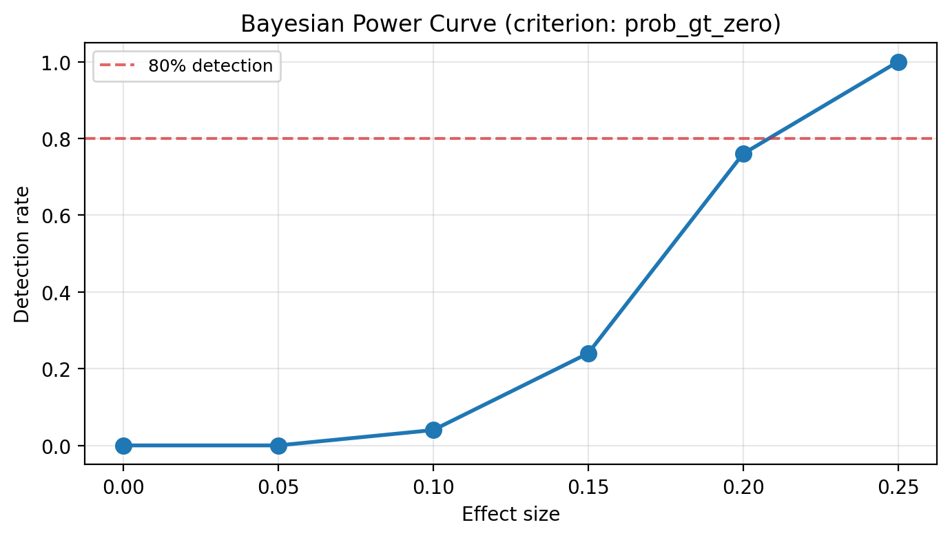
Abadie [2021] recommends an explicit go/no-go assessment before applying the synthetic control method. The power curve shows the probability of detecting an effect at each candidate size. If the curve crosses the 80% threshold at or below the effect size you expect (or the smallest effect that would justify the cost of the intervention), the design has adequate power and you can proceed with confidence.
If the curve stays below 80% at your target effect size, the experiment is underpowered. Common remedies include:
Extending the pre-period to give the model more data for learning donor weights. Ferman [2021] shows that the asymptotic properties of the SC estimator improve as the number of pre-treatment periods grows.
Adding donors that are more strongly correlated with the treated unit.
Lengthening the planned post-period, which accumulates a larger cumulative impact and makes detection easier.
For the Proposition 99 data, the effect of the tobacco tax on California’s cigarette sales was substantial — roughly a 25–30% decline relative to the synthetic control by 2000 [Abadie et al., 2010]. The power curve should confirm that this design can reliably detect effects well below that magnitude.
Tip
Before examining post-treatment data, document and commit to the SC specification — donor pool, matching variables, and pre-treatment period — as a form of pre-analysis plan. Ferman et al. [2020] show that the discretion inherent in choosing SC specifications creates “substantial room for specification searching,” and pre-commitment mitigates this risk.
Caveat — read the placebo-in-time check below before trusting this curve
The power curve above looks healthy at moderate effect sizes, but it inherits a residual bias from how validate_design constructs its pseudo-post window. Before treating the curve as the final word, see the placebo-in-time sanity check that follows — applying validate_design(injected_effect=0) to this design surfaces a structural identification problem with the donor pool that the power curve alone cannot reveal. The closing Putting it together section returns to this once all post-experiment robustness checks have run.
Placebo-in-time sanity check#
The power curve tells us how often the design detects a non-zero effect at a given magnitude. It does not tell us what the design infers when the true effect is zero. Calling validate_design(injected_effect=0, holdout_periods=5) on this design is mathematically equivalent to a single-fold placebo-in-time check on the pre-period: split the pre-period into a pseudo-pre and a pseudo-post window, refit the SC on the pseudo-pre, and measure the recovered cumulative impact across the pseudo-post window where — by construction — the true cumulative effect is zero.
This is conceptually the same diagnostic as the post-experiment placebo-in-time check below (see After the experiment: robustness and sensitivity → Placebo-in-time), just asked at a different stage of the workflow:
Design phase (now): can the SC reproduce California’s pre-treatment trajectory well enough that the recovered effect on a held-out pseudo-post window is near zero?
Post-experiment phase (later): does the same SC fit produce a near-zero impact when the intervention is reassigned to a placebo date in the pre-period?
If the donor pool can identify California’s trajectory shape across the full pre-period, we expect the recovered cumulative impact across the holdout window to sit near zero with the 94% HDI comfortably covering the truth.
rehearsal = design.validate_design(
    injected_effect=0,
    holdout_periods=5,
)

fig, ax = rehearsal.plot()
rehearsal.summary()
/Users/benjamv/git/CausalPy/causalpy/experiments/synthetic_control.py:128: UserWarning: Control units ['Connecticut' (r=-0.196), 'Kansas' (r=-0.211), 'Louisiana' (r=-0.126), 'Minnesota' (r=-0.201), 'Mississippi' (r=-0.195), 'North Dakota' (r=-0.155), 'Ohio' (r=-0.575), 'Oklahoma' (r=-0.230), 'Pennsylvania' (r=-0.416), 'South Carolina' (r=-0.014), 'Texas' (r=-0.405)] have pre-treatment correlation below 0.0 or undefined with treated unit 'California'. Consider excluding them from the donor pool. Use cp.plot_correlations() to inspect. See Abadie (2021) for guidance on donor pool selection.
  self._check_donor_correlations()
Initializing NUTS using jitter+adapt_diag...
Multiprocess sampling (4 chains in 4 jobs)
NUTS: [beta, y_hat_sigma]
Sampling 4 chains for 1_000 tune and 1_000 draw iterations (4_000 + 4_000 draws total) took 6 seconds.
Sampling: [beta, y_hat, y_hat_sigma]
Sampling: [y_hat]
Sampling: [y_hat]
Sampling: [y_hat]
Sampling: [y_hat]
| injected_effect | effect_type | injected_truth | recovered_mean | recovered_hdi_lower | recovered_hdi_upper | hdi_covers_truth | bias | relative_bias | |
|---|---|---|---|---|---|---|---|---|---|
| 0 | 0 | relative | 0.0 | -54.774385 | -75.05797 | -33.772227 | False | -54.774385 | NaN |
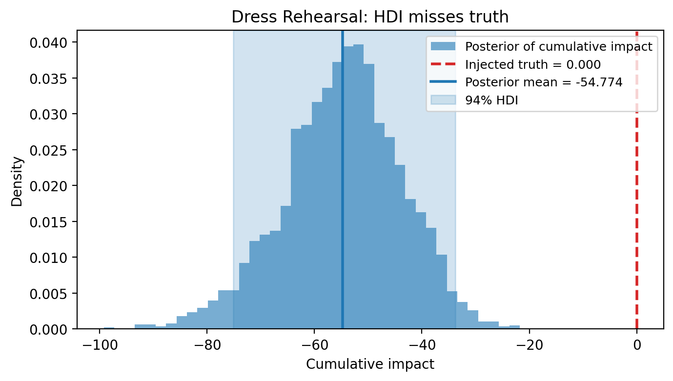
The result is unexpected. The recovered posterior mean is strongly negative and the 94% HDI excludes zero, so the design fails the placebo-in-time check at the design stage despite the power curve looking healthy. This is a structural finding rather than a sampling artefact: the donor pool cannot reproduce California’s trajectory shape across the full pre-period, and the synthetic control systematically over-predicts in the held-out window.
We will not attempt to fix this here. The post-experiment robustness suite below — placebo-in-space, placebo-in-time on the actual analysis, leave-one-out, prior sensitivity — gives multiple independent angles on whether this bias is fatal for the headline causal claim. We return to it in the closing Putting it together section at the end of the notebook.
After the experiment: estimating the causal effect#
The design assessment above would be done before running the experiment. Having confirmed the design is adequate, we now analyze the results after the intervention period. We fit the model on the full dataset — including both pre- and post-intervention observations — following the core SC estimation approach introduced by Abadie and Gardeazabal [2003] and Abadie et al. [2010]. The Bayesian formulation used here draws on Kim et al. [2020] for the prior structure and Brodersen et al. [2015] for the posterior predictive approach to causal impact.
For the Proposition 99 analysis, we expect to see California’s cigarette consumption diverge downward from its synthetic counterpart after the 1989 tax increase.
result = cp.SyntheticControl(
    df,
    treatment_time,
    control_units=control_units,
    treated_units=[treated_unit],
    model=cp.pymc_models.WeightedSumFitter(
        priors={
            "y_hat": Prior(
                "Normal",
                sigma=Prior("HalfNormal", sigma=10, dims=["treated_units"]),
                dims=["obs_ind", "treated_units"],
            ),
        },
        sample_kwargs={"target_accept": 0.95, "random_seed": seed},
    ),
)
Show code cell output
Initializing NUTS using jitter+adapt_diag...
Multiprocess sampling (4 chains in 4 jobs)
NUTS: [beta, y_hat_sigma]
Sampling 4 chains for 1_000 tune and 1_000 draw iterations (4_000 + 4_000 draws total) took 6 seconds.
Sampling: [beta, y_hat, y_hat_sigma]
Sampling: [y_hat]
Sampling: [y_hat]
Sampling: [y_hat]
Sampling: [y_hat]
fig, ax = result.plot(plot_predictors=True)
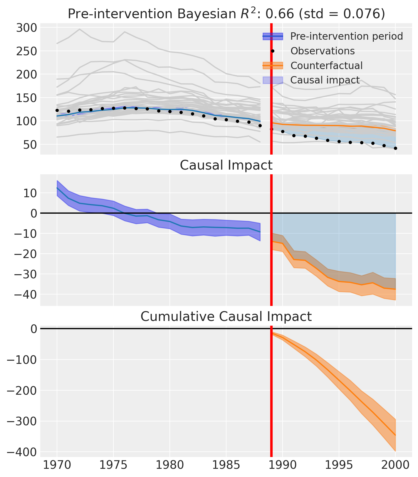
result.summary()
================================SyntheticControl================================
Control units: ['Colorado', 'Connecticut', 'Delaware', 'Idaho', 'Illinois', 'Indiana', 'Iowa', 'Kansas', 'Kentucky', 'Louisiana', 'Maine', 'Minnesota', 'Mississippi', 'Missouri', 'Montana', 'Nebraska', 'Nevada', 'New Hampshire', 'New Mexico', 'North Carolina', 'North Dakota', 'Ohio', 'Oklahoma', 'Pennsylvania', 'Rhode Island', 'South Carolina', 'South Dakota', 'Texas', 'Utah', 'Vermont', 'Virginia', 'West Virginia', 'Wisconsin', 'Wyoming']
Treated unit: California
Model coefficients:
    Colorado        0.036, 94% HDI [0.0014, 0.11]
    Connecticut     0.032, 94% HDI [0.00075, 0.11]
    Delaware        0.019, 94% HDI [0.00071, 0.065]
    Idaho           0.049, 94% HDI [0.0015, 0.16]
    Illinois        0.026, 94% HDI [0.0007, 0.092]
    Indiana         0.019, 94% HDI [0.00055, 0.064]
    Iowa            0.028, 94% HDI [0.00082, 0.1]
    Kansas          0.023, 94% HDI [0.00081, 0.077]
    Kentucky        0.0095, 94% HDI [0.00026, 0.034]
    Louisiana       0.019, 94% HDI [0.00048, 0.068]
    Maine           0.022, 94% HDI [0.00066, 0.075]
    Minnesota       0.028, 94% HDI [0.00069, 0.097]
    Mississippi     0.021, 94% HDI [0.00065, 0.071]
    Missouri        0.019, 94% HDI [0.00053, 0.066]
    Montana         0.044, 94% HDI [0.0016, 0.14]
    Nebraska        0.034, 94% HDI [0.0012, 0.12]
    Nevada          0.03, 94% HDI [0.00088, 0.098]
    New Hampshire   0.016, 94% HDI [0.00052, 0.052]
    New Mexico      0.061, 94% HDI [0.0016, 0.2]
    North Carolina  0.02, 94% HDI [0.00072, 0.063]
    North Dakota    0.026, 94% HDI [0.00067, 0.091]
    Ohio            0.02, 94% HDI [0.00051, 0.072]
    Oklahoma        0.018, 94% HDI [0.00055, 0.063]
    Pennsylvania    0.022, 94% HDI [0.00073, 0.076]
    Rhode Island    0.017, 94% HDI [0.00053, 0.056]
    South Carolina  0.017, 94% HDI [0.00056, 0.06]
    South Dakota    0.029, 94% HDI [0.00075, 0.11]
    Texas           0.022, 94% HDI [0.00068, 0.079]
    Utah            0.16, 94% HDI [0.03, 0.3]
    Vermont         0.014, 94% HDI [0.00051, 0.05]
    Virginia        0.017, 94% HDI [0.00056, 0.058]
    West Virginia   0.029, 94% HDI [0.00079, 0.1]
    Wisconsin       0.031, 94% HDI [0.001, 0.11]
    Wyoming         0.019, 94% HDI [0.00051, 0.068]
    y_hat_sigma     6.8, 94% HDI [4.4, 10]
Pre-treatment correlation (California): 0.8610
We can get nicely formatted tables from our integration with the maketables package.
from maketables import ETable

result.set_maketables_options(hdi_prob=0.95)
ETable(result, coef_fmt="b:.3f \n [ci95l:.3f, ci95u:.3f]")
| y | |
|---|---|
| (1) | |
| coef | |
| Colorado | 0.036 [0.000, 0.102] |
| Connecticut | 0.032 [0.000, 0.095] |
| Delaware | 0.019 [0.000, 0.056] |
| Idaho | 0.049 [0.000, 0.139] |
| Illinois | 0.026 [0.000, 0.077] |
| Indiana | 0.019 [0.000, 0.056] |
| Iowa | 0.028 [0.000, 0.087] |
| Kansas | 0.023 [0.000, 0.066] |
| Kentucky | 0.009 [0.000, 0.029] |
| Louisiana | 0.019 [0.000, 0.058] |
| Maine | 0.022 [0.000, 0.063] |
| Minnesota | 0.028 [0.000, 0.085] |
| Mississippi | 0.021 [0.000, 0.060] |
| Missouri | 0.019 [0.000, 0.056] |
| Montana | 0.044 [0.000, 0.127] |
| Nebraska | 0.034 [0.000, 0.102] |
| Nevada | 0.030 [0.000, 0.085] |
| New Hampshire | 0.016 [0.000, 0.045] |
| New Mexico | 0.061 [0.000, 0.181] |
| North Carolina | 0.020 [0.000, 0.057] |
| North Dakota | 0.026 [0.000, 0.078] |
| Ohio | 0.020 [0.000, 0.061] |
| Oklahoma | 0.018 [0.000, 0.055] |
| Pennsylvania | 0.022 [0.000, 0.065] |
| Rhode Island | 0.017 [0.000, 0.049] |
| South Carolina | 0.017 [0.000, 0.051] |
| South Dakota | 0.029 [0.000, 0.090] |
| Texas | 0.022 [0.000, 0.064] |
| Utah | 0.164 [0.007, 0.288] |
| Vermont | 0.014 [0.000, 0.043] |
| Virginia | 0.017 [0.000, 0.050] |
| West Virginia | 0.029 [0.000, 0.089] |
| Wisconsin | 0.031 [0.000, 0.093] |
| Wyoming | 0.019 [0.000, 0.060] |
| stats | |
| N | 31 |
| Bayesian R2 | 0.663 |
| Format of coefficient cell: Coefficient [95% CI Lower, 95% CI Upper] | |
As well as the model coefficients, we might be interested in the average causal impact and average cumulative causal impact. The posterior predictive approach to pointwise and cumulative effects follows Brodersen et al. [2015], while Cattaneo et al. [2021] provide the theoretical foundation for prediction intervals in the SC framework.
az.summary(result.post_impact.mean("obs_ind"))
| mean | sd | hdi_3% | hdi_97% | mcse_mean | mcse_sd | ess_bulk | ess_tail | r_hat | |
|---|---|---|---|---|---|---|---|---|---|
| x[California] | -28.802 | 2.326 | -33.143 | -24.528 | 0.038 | 0.033 | 3951.0 | 3128.0 | 1.0 |
Warning
Care must be taken with the mean impact statistic. It only makes sense to use this statistic if it looks like the intervention had a lasting (and roughly constant) effect on the outcome variable. If the effect is transient, then clearly there will be a lot of post-intervention period where the impact of the intervention has ‘worn off’. If so, then it will be hard to interpret the mean impacts real meaning.
We can also ask for the summary statistics of the cumulative causal impact.
# get index of the final time point
index = result.post_impact_cumulative.obs_ind.max()
# grab the posterior distribution of the cumulative impact at this final time point
last_cumulative_estimate = result.post_impact_cumulative.sel({"obs_ind": index})
# get summary stats
az.summary(last_cumulative_estimate)
| mean | sd | hdi_3% | hdi_97% | mcse_mean | mcse_sd | ess_bulk | ess_tail | r_hat | |
|---|---|---|---|---|---|---|---|---|---|
| x[California] | -345.62 | 27.913 | -397.722 | -294.333 | 0.45 | 0.394 | 3951.0 | 3128.0 | 1.0 |
Decision-ready effect summary#
For decision-making, you often need a concise summary of the causal effect with key statistics. Brodersen et al. [2015] produce exactly this type of summary — posterior probability of a causal effect, cumulative impact with credible intervals, and relative effect sizes — and Abadie [2021] recommends reporting effect estimates alongside measures of uncertainty and significance. The effect_summary() method provides this decision-ready report with average and cumulative effects, HDI intervals, tail probabilities, and relative effects.
stats = result.effect_summary(treated_unit=treated_unit)
stats.table
| mean | median | hdi_lower | hdi_upper | p_gt_0 | relative_mean | relative_hdi_lower | relative_hdi_upper | |
|---|---|---|---|---|---|---|---|---|
| average | -28.801688 | -28.693411 | -33.400530 | -24.399117 | 0.0 | -32.260575 | -35.719528 | -28.89775 |
| cumulative | -345.620259 | -344.320926 | -400.806366 | -292.789406 | 0.0 | -32.260575 | -35.719528 | -28.89775 |
print(stats.text)
During the Post-period (1989 to 2000), the response variable had an average value of approx. 60.35. By contrast, in the absence of an intervention, we would have expected an average response of 89.15. The 95% interval of this counterfactual prediction is [84.75, 93.75]. Subtracting this prediction from the observed response yields an estimate of the causal effect the intervention had on the response variable. This effect is -28.80 with a 95% interval of [-33.40, -24.40].

Summing up the individual data points during the Post-period, the response variable had an overall value of 724.20. By contrast, had the intervention not taken place, we would have expected a sum of 1069.82. The 95% interval of this prediction is [1016.99, 1125.01].

The 95% HDI of the effect [-33.40, -24.40] does not include zero. The posterior probability of a decrease is 1.000. Relative to the counterfactual, the effect represents a -32.26% change (95% HDI [-35.72%, -28.90%]).

This analysis assumes that the control units used to construct the synthetic counterfactual were not themselves affected by the intervention, and that the pre-treatment relationship between control and treated units remains stable throughout the post-treatment period. We recommend inspecting model fit, examining pre-intervention trends, and conducting sensitivity analyses (e.g., placebo tests) to support any causal conclusions drawn from this analysis.
You can customize the summary in several ways:
Window: Analyze a specific time period instead of the full post-period
Direction: Specify whether you’re testing for an increase, decrease, or two-sided effect
Options: Include/exclude cumulative or relative effects
post_indices = result.datapost.index
window_start = post_indices[0]
window_end = post_indices[len(post_indices) // 2]

stats_windowed = result.effect_summary(
    window=(window_start, window_end),
    treated_unit=treated_unit,
    direction="two-sided",
    cumulative=True,
    relative=True,
)

stats_windowed.table
| mean | median | hdi_lower | hdi_upper | p_two_sided | prob_of_effect | relative_mean | relative_hdi_lower | relative_hdi_upper | |
|---|---|---|---|---|---|---|---|---|---|
| average | -23.912950 | -23.803696 | -28.131407 | -19.779764 | 0.0 | 1.0 | -26.024751 | -29.31577 | -22.577491 |
| cumulative | -167.390648 | -166.625869 | -196.919848 | -138.458351 | 0.0 | 1.0 | -26.024751 | -29.31577 | -22.577491 |
print(stats_windowed.text)
During the Post-period (1989 to 1995), the response variable had an average value of approx. 67.83. By contrast, in the absence of an intervention, we would have expected an average response of 91.74. The 95% interval of this counterfactual prediction is [87.61, 95.96]. Subtracting this prediction from the observed response yields an estimate of the causal effect the intervention had on the response variable. This effect is -23.91 with a 95% interval of [-28.13, -19.78].

Summing up the individual data points during the Post-period, the response variable had an overall value of 474.80. By contrast, had the intervention not taken place, we would have expected a sum of 642.19. The 95% interval of this prediction is [613.26, 671.72].

The 95% HDI of the effect [-28.13, -19.78] does not include zero. The posterior probability of an effect is 1.000. Relative to the counterfactual, the effect represents a -26.02% change (95% HDI [-29.32%, -22.58%]).

This analysis assumes that the control units used to construct the synthetic counterfactual were not themselves affected by the intervention, and that the pre-treatment relationship between control and treated units remains stable throughout the post-treatment period. We recommend inspecting model fit, examining pre-intervention trends, and conducting sensitivity analyses (e.g., placebo tests) to support any causal conclusions drawn from this analysis.
After the experiment: robustness and sensitivity#
Estimation alone does not establish a causal claim. The SC literature strongly recommends a battery of post-estimation robustness checks to probe the reliability of the effect estimate from different angles [Abadie et al., 2010, Abadie et al., 2015, Athey and Imbens, 2017]. If the estimated effect survives these checks, we can be more confident it reflects a genuine causal effect rather than an artefact of the particular model specification, donor pool composition, or prior assumptions.
The four checks below cover the primary threats to SC validity:
Placebo-in-space — does the effect stand out relative to placebo effects estimated for control units?
Placebo-in-time — does the model show a spurious effect when the intervention is reassigned to a pre-period date?
Leave-one-out — is the effect driven by a single donor unit?
Prior sensitivity — are the posterior conclusions dominated by the Bayesian prior?
CausalPy implements all four as Check objects that can be run individually or together via SensitivityAnalysis.
from causalpy.pipeline import PipelineContext

context = PipelineContext(
    data=df,
    experiment=result,
    experiment_config={
        "method": cp.SyntheticControl,
        "treatment_time": treatment_time,
        "control_units": control_units,
        "treated_units": [treated_unit],
        "model": cp.pymc_models.WeightedSumFitter(
            priors={
                "y_hat": Prior(
                    "Normal",
                    sigma=Prior("HalfNormal", sigma=10, dims=["treated_units"]),
                    dims=["obs_ind", "treated_units"],
                ),
            },
            sample_kwargs={"target_accept": 0.95, "random_seed": seed},
        ),
    },
)
Placebo-in-space#
The placebo-in-space test is the primary inference tool for synthetic control, introduced by Abadie et al. [2010] and further developed by Abadie et al. [2015]. The idea is simple: reassign treatment to each control state in turn, fit a separate SC for each using the remaining states as donors, and compare the resulting placebo effects to the actual estimated effect for California. If placebo effects are frequently as large as the real one, the estimated treatment effect is not distinguishable from noise, and the causal claim is weakened.
Ferman and Pinto [2017] analyse the statistical properties of this permutation-based inference approach and show that while it can have size distortions in small donor pools, it remains the most widely used inference tool for SC. With 38 donor states, this test is well-powered. Firpo and Possebom [2018] extend the framework by allowing non-uniform treatment assignment probabilities and constructing formal confidence sets.
Note
With 38 control states, this step fits 38 separate SC models — one per placebo assignment. This may take a few minutes.
from causalpy.checks import PlaceboInSpace

pis_check = PlaceboInSpace()
pis_result = pis_check.run(result, context)
Show code cell output
Initializing NUTS using jitter+adapt_diag...
Multiprocess sampling (4 chains in 4 jobs)
NUTS: [beta, y_hat_sigma]
Sampling 4 chains for 1_000 tune and 1_000 draw iterations (4_000 + 4_000 draws total) took 7 seconds.
Sampling: [beta, y_hat, y_hat_sigma]
Sampling: [y_hat]
Sampling: [y_hat]
Sampling: [y_hat]
Sampling: [y_hat]
Initializing NUTS using jitter+adapt_diag...
Multiprocess sampling (4 chains in 4 jobs)
NUTS: [beta, y_hat_sigma]
Sampling 4 chains for 1_000 tune and 1_000 draw iterations (4_000 + 4_000 draws total) took 6 seconds.
Sampling: [beta, y_hat, y_hat_sigma]
Sampling: [y_hat]
Sampling: [y_hat]
Sampling: [y_hat]
Sampling: [y_hat]
/Users/benjamv/git/CausalPy/causalpy/experiments/synthetic_control.py:128: UserWarning: Control units ['South Carolina' (r=-0.069)] have pre-treatment correlation below 0.0 or undefined with treated unit 'Delaware'. Consider excluding them from the donor pool. Use cp.plot_correlations() to inspect. See Abadie (2021) for guidance on donor pool selection.
  self._check_donor_correlations()
Initializing NUTS using jitter+adapt_diag...
Multiprocess sampling (4 chains in 4 jobs)
NUTS: [beta, y_hat_sigma]
Sampling 4 chains for 1_000 tune and 1_000 draw iterations (4_000 + 4_000 draws total) took 5 seconds.
Sampling: [beta, y_hat, y_hat_sigma]
Sampling: [y_hat]
Sampling: [y_hat]
Sampling: [y_hat]
Sampling: [y_hat]
Initializing NUTS using jitter+adapt_diag...
Multiprocess sampling (4 chains in 4 jobs)
NUTS: [beta, y_hat_sigma]
Sampling 4 chains for 1_000 tune and 1_000 draw iterations (4_000 + 4_000 draws total) took 6 seconds.
Sampling: [beta, y_hat, y_hat_sigma]
Sampling: [y_hat]
Sampling: [y_hat]
Sampling: [y_hat]
Sampling: [y_hat]
Initializing NUTS using jitter+adapt_diag...
Multiprocess sampling (4 chains in 4 jobs)
NUTS: [beta, y_hat_sigma]
Sampling 4 chains for 1_000 tune and 1_000 draw iterations (4_000 + 4_000 draws total) took 10 seconds.
Sampling: [beta, y_hat, y_hat_sigma]
Sampling: [y_hat]
Sampling: [y_hat]
Sampling: [y_hat]
Sampling: [y_hat]
/Users/benjamv/git/CausalPy/causalpy/experiments/synthetic_control.py:128: UserWarning: Control units ['Ohio' (r=-0.022)] have pre-treatment correlation below 0.0 or undefined with treated unit 'Indiana'. Consider excluding them from the donor pool. Use cp.plot_correlations() to inspect. See Abadie (2021) for guidance on donor pool selection.
  self._check_donor_correlations()
Initializing NUTS using jitter+adapt_diag...
Multiprocess sampling (4 chains in 4 jobs)
NUTS: [beta, y_hat_sigma]
Sampling 4 chains for 1_000 tune and 1_000 draw iterations (4_000 + 4_000 draws total) took 6 seconds.
Sampling: [beta, y_hat, y_hat_sigma]
Sampling: [y_hat]
Sampling: [y_hat]
Sampling: [y_hat]
Sampling: [y_hat]
Initializing NUTS using jitter+adapt_diag...
Multiprocess sampling (4 chains in 4 jobs)
NUTS: [beta, y_hat_sigma]
Sampling 4 chains for 1_000 tune and 1_000 draw iterations (4_000 + 4_000 draws total) took 11 seconds.
There was 1 divergence after tuning. Increase `target_accept` or reparameterize.
Sampling: [beta, y_hat, y_hat_sigma]
Sampling: [y_hat]
Sampling: [y_hat]
Sampling: [y_hat]
Sampling: [y_hat]
Initializing NUTS using jitter+adapt_diag...
Multiprocess sampling (4 chains in 4 jobs)
NUTS: [beta, y_hat_sigma]
Sampling 4 chains for 1_000 tune and 1_000 draw iterations (4_000 + 4_000 draws total) took 7 seconds.
Sampling: [beta, y_hat, y_hat_sigma]
Sampling: [y_hat]
Sampling: [y_hat]
Sampling: [y_hat]
Sampling: [y_hat]
Initializing NUTS using jitter+adapt_diag...
Multiprocess sampling (4 chains in 4 jobs)
NUTS: [beta, y_hat_sigma]
Sampling 4 chains for 1_000 tune and 1_000 draw iterations (4_000 + 4_000 draws total) took 4 seconds.
Sampling: [beta, y_hat, y_hat_sigma]
Sampling: [y_hat]
Sampling: [y_hat]
Sampling: [y_hat]
Sampling: [y_hat]
Initializing NUTS using jitter+adapt_diag...
Multiprocess sampling (4 chains in 4 jobs)
NUTS: [beta, y_hat_sigma]
Sampling 4 chains for 1_000 tune and 1_000 draw iterations (4_000 + 4_000 draws total) took 11 seconds.
Sampling: [beta, y_hat, y_hat_sigma]
Sampling: [y_hat]
Sampling: [y_hat]
Sampling: [y_hat]
Sampling: [y_hat]
Initializing NUTS using jitter+adapt_diag...
Multiprocess sampling (4 chains in 4 jobs)
NUTS: [beta, y_hat_sigma]
Sampling 4 chains for 1_000 tune and 1_000 draw iterations (4_000 + 4_000 draws total) took 7 seconds.
Sampling: [beta, y_hat, y_hat_sigma]
Sampling: [y_hat]
Sampling: [y_hat]
Sampling: [y_hat]
Sampling: [y_hat]
Initializing NUTS using jitter+adapt_diag...
Multiprocess sampling (4 chains in 4 jobs)
NUTS: [beta, y_hat_sigma]
Sampling 4 chains for 1_000 tune and 1_000 draw iterations (4_000 + 4_000 draws total) took 6 seconds.
Sampling: [beta, y_hat, y_hat_sigma]
Sampling: [y_hat]
Sampling: [y_hat]
Sampling: [y_hat]
Sampling: [y_hat]
Initializing NUTS using jitter+adapt_diag...
Multiprocess sampling (4 chains in 4 jobs)
NUTS: [beta, y_hat_sigma]
Sampling 4 chains for 1_000 tune and 1_000 draw iterations (4_000 + 4_000 draws total) took 7 seconds.
Sampling: [beta, y_hat, y_hat_sigma]
Sampling: [y_hat]
Sampling: [y_hat]
Sampling: [y_hat]
Sampling: [y_hat]
Initializing NUTS using jitter+adapt_diag...
Multiprocess sampling (4 chains in 4 jobs)
NUTS: [beta, y_hat_sigma]
Sampling 4 chains for 1_000 tune and 1_000 draw iterations (4_000 + 4_000 draws total) took 10 seconds.
Sampling: [beta, y_hat, y_hat_sigma]
Sampling: [y_hat]
Sampling: [y_hat]
Sampling: [y_hat]
Sampling: [y_hat]
/Users/benjamv/git/CausalPy/causalpy/experiments/synthetic_control.py:128: UserWarning: Control units ['Ohio' (r=-0.259), 'Pennsylvania' (r=-0.040)] have pre-treatment correlation below 0.0 or undefined with treated unit 'Nevada'. Consider excluding them from the donor pool. Use cp.plot_correlations() to inspect. See Abadie (2021) for guidance on donor pool selection.
  self._check_donor_correlations()
Initializing NUTS using jitter+adapt_diag...
Multiprocess sampling (4 chains in 4 jobs)
NUTS: [beta, y_hat_sigma]
Sampling 4 chains for 1_000 tune and 1_000 draw iterations (4_000 + 4_000 draws total) took 6 seconds.
Sampling: [beta, y_hat, y_hat_sigma]
Sampling: [y_hat]
Sampling: [y_hat]
Sampling: [y_hat]
Sampling: [y_hat]
/Users/benjamv/git/CausalPy/causalpy/experiments/synthetic_control.py:128: UserWarning: Control units ['Ohio' (r=-0.113)] have pre-treatment correlation below 0.0 or undefined with treated unit 'New Hampshire'. Consider excluding them from the donor pool. Use cp.plot_correlations() to inspect. See Abadie (2021) for guidance on donor pool selection.
  self._check_donor_correlations()
/Users/benjamv/git/CausalPy/causalpy/experiments/synthetic_control.py:129: UserWarning: Convex hull assumption may be violated: 19 pre-intervention time points (100.0% above, 0.0% below control range). The synthetic control method requires the treated unit to lie within the convex hull of control units. Consider: (1) adding more diverse control units, (2) using a model with an intercept (e.g., ITS with control predictors), or (3) using the Augmented Synthetic Control Method. See glossary term 'Convex hull condition' for more details.
  self._check_convex_hull()
Initializing NUTS using jitter+adapt_diag...
Multiprocess sampling (4 chains in 4 jobs)
NUTS: [beta, y_hat_sigma]
Sampling 4 chains for 1_000 tune and 1_000 draw iterations (4_000 + 4_000 draws total) took 4 seconds.
Sampling: [beta, y_hat, y_hat_sigma]
Sampling: [y_hat]
Sampling: [y_hat]
Sampling: [y_hat]
Sampling: [y_hat]
Initializing NUTS using jitter+adapt_diag...
Multiprocess sampling (4 chains in 4 jobs)
NUTS: [beta, y_hat_sigma]
Sampling 4 chains for 1_000 tune and 1_000 draw iterations (4_000 + 4_000 draws total) took 11 seconds.
Sampling: [beta, y_hat, y_hat_sigma]
Sampling: [y_hat]
Sampling: [y_hat]
Sampling: [y_hat]
Sampling: [y_hat]
/Users/benjamv/git/CausalPy/causalpy/experiments/synthetic_control.py:128: UserWarning: Control units ['Ohio' (r=-0.194)] have pre-treatment correlation below 0.0 or undefined with treated unit 'North Carolina'. Consider excluding them from the donor pool. Use cp.plot_correlations() to inspect. See Abadie (2021) for guidance on donor pool selection.
  self._check_donor_correlations()
Initializing NUTS using jitter+adapt_diag...
Multiprocess sampling (4 chains in 4 jobs)
NUTS: [beta, y_hat_sigma]
Sampling 4 chains for 1_000 tune and 1_000 draw iterations (4_000 + 4_000 draws total) took 5 seconds.
Sampling: [beta, y_hat, y_hat_sigma]
Sampling: [y_hat]
Sampling: [y_hat]
Sampling: [y_hat]
Sampling: [y_hat]
Initializing NUTS using jitter+adapt_diag...
Multiprocess sampling (4 chains in 4 jobs)
NUTS: [beta, y_hat_sigma]
Sampling 4 chains for 1_000 tune and 1_000 draw iterations (4_000 + 4_000 draws total) took 7 seconds.
Sampling: [beta, y_hat, y_hat_sigma]
Sampling: [y_hat]
Sampling: [y_hat]
Sampling: [y_hat]
Sampling: [y_hat]
/Users/benjamv/git/CausalPy/causalpy/experiments/synthetic_control.py:128: UserWarning: Control units ['Indiana' (r=-0.022), 'Nevada' (r=-0.259), 'New Hampshire' (r=-0.113), 'North Carolina' (r=-0.194)] have pre-treatment correlation below 0.0 or undefined with treated unit 'Ohio'. Consider excluding them from the donor pool. Use cp.plot_correlations() to inspect. See Abadie (2021) for guidance on donor pool selection.
  self._check_donor_correlations()
Initializing NUTS using jitter+adapt_diag...
Multiprocess sampling (4 chains in 4 jobs)
NUTS: [beta, y_hat_sigma]
Sampling 4 chains for 1_000 tune and 1_000 draw iterations (4_000 + 4_000 draws total) took 5 seconds.
Sampling: [beta, y_hat, y_hat_sigma]
Sampling: [y_hat]
Sampling: [y_hat]
Sampling: [y_hat]
Sampling: [y_hat]
Initializing NUTS using jitter+adapt_diag...
Multiprocess sampling (4 chains in 4 jobs)
NUTS: [beta, y_hat_sigma]
Sampling 4 chains for 1_000 tune and 1_000 draw iterations (4_000 + 4_000 draws total) took 6 seconds.
Sampling: [beta, y_hat, y_hat_sigma]
Sampling: [y_hat]
Sampling: [y_hat]
Sampling: [y_hat]
Sampling: [y_hat]
/Users/benjamv/git/CausalPy/causalpy/experiments/synthetic_control.py:128: UserWarning: Control units ['Nevada' (r=-0.040)] have pre-treatment correlation below 0.0 or undefined with treated unit 'Pennsylvania'. Consider excluding them from the donor pool. Use cp.plot_correlations() to inspect. See Abadie (2021) for guidance on donor pool selection.
  self._check_donor_correlations()
Initializing NUTS using jitter+adapt_diag...
Multiprocess sampling (4 chains in 4 jobs)
NUTS: [beta, y_hat_sigma]
Sampling 4 chains for 1_000 tune and 1_000 draw iterations (4_000 + 4_000 draws total) took 6 seconds.
There were 2 divergences after tuning. Increase `target_accept` or reparameterize.
Sampling: [beta, y_hat, y_hat_sigma]
Sampling: [y_hat]
Sampling: [y_hat]
Sampling: [y_hat]
Sampling: [y_hat]
Initializing NUTS using jitter+adapt_diag...
Multiprocess sampling (4 chains in 4 jobs)
NUTS: [beta, y_hat_sigma]
Sampling 4 chains for 1_000 tune and 1_000 draw iterations (4_000 + 4_000 draws total) took 5 seconds.
Sampling: [beta, y_hat, y_hat_sigma]
Sampling: [y_hat]
Sampling: [y_hat]
Sampling: [y_hat]
Sampling: [y_hat]
/Users/benjamv/git/CausalPy/causalpy/experiments/synthetic_control.py:128: UserWarning: Control units ['Delaware' (r=-0.069)] have pre-treatment correlation below 0.0 or undefined with treated unit 'South Carolina'. Consider excluding them from the donor pool. Use cp.plot_correlations() to inspect. See Abadie (2021) for guidance on donor pool selection.
  self._check_donor_correlations()
Initializing NUTS using jitter+adapt_diag...
Multiprocess sampling (4 chains in 4 jobs)
NUTS: [beta, y_hat_sigma]
Sampling 4 chains for 1_000 tune and 1_000 draw iterations (4_000 + 4_000 draws total) took 6 seconds.
Sampling: [beta, y_hat, y_hat_sigma]
Sampling: [y_hat]
Sampling: [y_hat]
Sampling: [y_hat]
Sampling: [y_hat]
Initializing NUTS using jitter+adapt_diag...
Multiprocess sampling (4 chains in 4 jobs)
NUTS: [beta, y_hat_sigma]
Sampling 4 chains for 1_000 tune and 1_000 draw iterations (4_000 + 4_000 draws total) took 11 seconds.
There was 1 divergence after tuning. Increase `target_accept` or reparameterize.
Sampling: [beta, y_hat, y_hat_sigma]
Sampling: [y_hat]
Sampling: [y_hat]
Sampling: [y_hat]
Sampling: [y_hat]
Initializing NUTS using jitter+adapt_diag...
Multiprocess sampling (4 chains in 4 jobs)
NUTS: [beta, y_hat_sigma]
Sampling 4 chains for 1_000 tune and 1_000 draw iterations (4_000 + 4_000 draws total) took 6 seconds.
There was 1 divergence after tuning. Increase `target_accept` or reparameterize.
Sampling: [beta, y_hat, y_hat_sigma]
Sampling: [y_hat]
Sampling: [y_hat]
Sampling: [y_hat]
Sampling: [y_hat]
/Users/benjamv/git/CausalPy/causalpy/experiments/synthetic_control.py:129: UserWarning: Convex hull assumption may be violated: 19 pre-intervention time points (0.0% above, 100.0% below control range). The synthetic control method requires the treated unit to lie within the convex hull of control units. Consider: (1) adding more diverse control units, (2) using a model with an intercept (e.g., ITS with control predictors), or (3) using the Augmented Synthetic Control Method. See glossary term 'Convex hull condition' for more details.
  self._check_convex_hull()
Initializing NUTS using jitter+adapt_diag...
Multiprocess sampling (4 chains in 4 jobs)
NUTS: [beta, y_hat_sigma]
Sampling 4 chains for 1_000 tune and 1_000 draw iterations (4_000 + 4_000 draws total) took 4 seconds.
Sampling: [beta, y_hat, y_hat_sigma]
Sampling: [y_hat]
Sampling: [y_hat]
Sampling: [y_hat]
Sampling: [y_hat]
Initializing NUTS using jitter+adapt_diag...
Multiprocess sampling (4 chains in 4 jobs)
NUTS: [beta, y_hat_sigma]
Sampling 4 chains for 1_000 tune and 1_000 draw iterations (4_000 + 4_000 draws total) took 6 seconds.
Sampling: [beta, y_hat, y_hat_sigma]
Sampling: [y_hat]
Sampling: [y_hat]
Sampling: [y_hat]
Sampling: [y_hat]
Initializing NUTS using jitter+adapt_diag...
Multiprocess sampling (4 chains in 4 jobs)
NUTS: [beta, y_hat_sigma]
Sampling 4 chains for 1_000 tune and 1_000 draw iterations (4_000 + 4_000 draws total) took 7 seconds.
Sampling: [beta, y_hat, y_hat_sigma]
Sampling: [y_hat]
Sampling: [y_hat]
Sampling: [y_hat]
Sampling: [y_hat]
Initializing NUTS using jitter+adapt_diag...
Multiprocess sampling (4 chains in 4 jobs)
NUTS: [beta, y_hat_sigma]
Sampling 4 chains for 1_000 tune and 1_000 draw iterations (4_000 + 4_000 draws total) took 6 seconds.
Sampling: [beta, y_hat, y_hat_sigma]
Sampling: [y_hat]
Sampling: [y_hat]
Sampling: [y_hat]
Sampling: [y_hat]
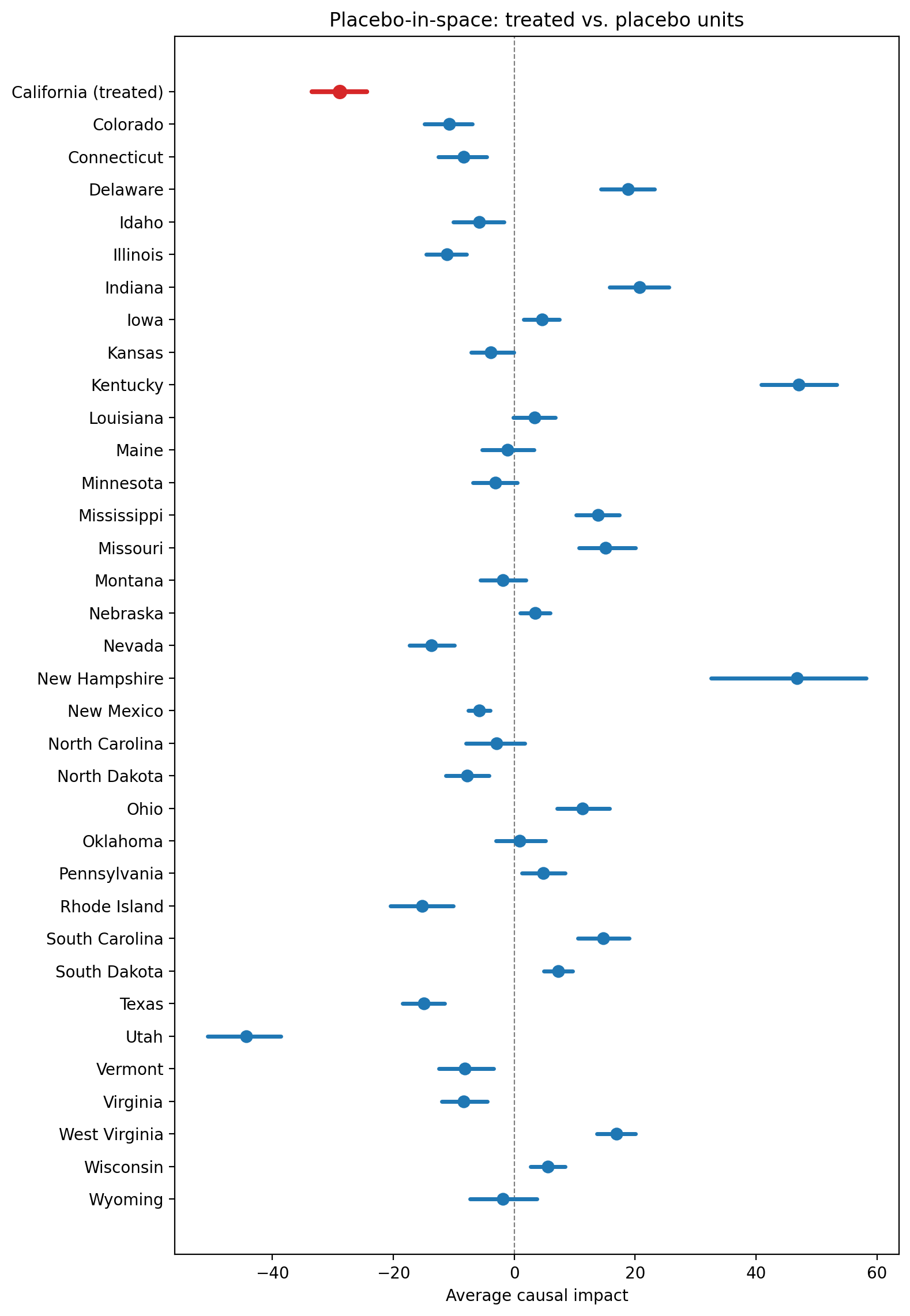
print(pis_result.text)
Placebo-in-space analysis: tested 34 control units as placebo treated units. If placebo effects are comparable to the actual effect, the causal claim may be weakened.
pis_result.table
| placebo_treated | mean | median | hdi_lower | hdi_upper | p_gt_0 | relative_mean | relative_hdi_lower | relative_hdi_upper | |
|---|---|---|---|---|---|---|---|---|---|
| 0 | Colorado | -10.728776 | -10.661444 | -14.815481 | -6.918418 | 0.00000 | -11.205242 | -14.892602 | -7.554088 |
| 1 | Connecticut | -8.389137 | -8.302533 | -12.585296 | -4.557407 | 0.00000 | -9.356998 | -13.477946 | -5.339726 |
| 2 | Delaware | 18.817058 | 18.844172 | 14.317429 | 23.220651 | 1.00000 | 17.227937 | 12.555561 | 22.087696 |
| 3 | Idaho | -5.766426 | -5.602764 | -10.041019 | -1.631898 | 0.00150 | -6.622328 | -11.129350 | -2.030465 |
| 4 | Illinois | -11.129919 | -11.088901 | -14.572083 | -7.872692 | 0.00000 | -11.371551 | -14.416327 | -8.341392 |
| 5 | Indiana | 20.744293 | 20.872401 | 15.756954 | 25.603179 | 1.00000 | 18.882209 | 13.658083 | 24.279203 |
| 6 | Iowa | 4.661463 | 4.689598 | 1.578932 | 7.494899 | 0.99800 | 5.271678 | 1.715372 | 8.701834 |
| 7 | Kansas | -3.887174 | -3.858994 | -7.126898 | -0.045865 | 0.01450 | -4.140540 | -7.870148 | -0.554248 |
| 8 | Kentucky | 47.002523 | 46.757117 | 40.834864 | 53.321849 | 1.00000 | 37.703592 | 30.881231 | 44.655310 |
| 9 | Louisiana | 3.387238 | 3.386568 | -0.160445 | 6.840617 | 0.97150 | 3.368558 | -0.243672 | 6.885723 |
| 10 | Maine | -1.140612 | -1.124624 | -5.266424 | 3.292558 | 0.29325 | -1.043667 | -5.046000 | 3.018254 |
| 11 | Minnesota | -3.121289 | -3.039172 | -6.835969 | 0.472414 | 0.03975 | -3.539472 | -7.527000 | 0.565691 |
| 12 | Mississippi | 13.818726 | 13.848917 | 10.226307 | 17.371102 | 1.00000 | 15.204268 | 10.792136 | 19.827256 |
| 13 | Missouri | 15.150447 | 15.116985 | 10.671529 | 20.041794 | 1.00000 | 14.446698 | 9.422277 | 19.606259 |
| 14 | Montana | -1.852976 | -1.751924 | -5.593833 | 1.952743 | 0.16400 | -2.068957 | -6.388409 | 2.056251 |
| 15 | Nebraska | 3.515486 | 3.538452 | 0.990175 | 5.917005 | 0.99475 | 4.205494 | 1.143259 | 7.243864 |
| 16 | Nevada | -13.662526 | -13.622196 | -17.286429 | -9.842517 | 0.00000 | -11.109375 | -13.679245 | -8.276180 |
| 17 | New Hampshire | 46.746848 | 47.513274 | 32.551941 | 58.157126 | 1.00000 | 42.393998 | 25.876346 | 58.045171 |
| 18 | New Mexico | -5.750467 | -5.707787 | -7.573022 | -3.992418 | 0.00000 | -7.978164 | -10.266459 | -5.688494 |
| 19 | North Carolina | -2.956831 | -2.956378 | -7.983112 | 1.759413 | 0.10500 | -2.266033 | -5.983230 | 1.422527 |
| 20 | North Dakota | -7.754787 | -7.677051 | -11.330950 | -4.125011 | 0.00000 | -8.881034 | -12.613693 | -5.054236 |
| 21 | Ohio | 11.245835 | 11.276261 | 7.135396 | 15.733044 | 1.00000 | 11.489238 | 6.762435 | 16.556450 |
| 22 | Oklahoma | 0.915472 | 0.923308 | -2.986338 | 5.216840 | 0.67425 | 0.956086 | -3.209721 | 5.040448 |
| 23 | Pennsylvania | 4.810412 | 4.869477 | 1.251304 | 8.409518 | 0.99325 | 5.329979 | 1.179236 | 9.475531 |
| 24 | Rhode Island | -15.211598 | -15.382465 | -20.454279 | -10.053766 | 0.00000 | -13.761831 | -17.730423 | -9.578473 |
| 25 | South Carolina | 14.725585 | 14.754356 | 10.514923 | 19.015725 | 1.00000 | 14.745252 | 10.067579 | 19.819896 |
| 26 | South Dakota | 7.271180 | 7.300218 | 4.870692 | 9.624013 | 1.00000 | 8.871089 | 5.758160 | 12.054982 |
| 27 | Texas | -14.901892 | -14.858505 | -18.417665 | -11.499270 | 0.00000 | -16.107250 | -19.213220 | -12.929109 |
| 28 | Utah | -44.291970 | -44.234391 | -50.645984 | -38.561986 | 0.00000 | -46.070855 | -49.568936 | -42.825429 |
| 29 | Vermont | -8.151271 | -8.382257 | -12.466818 | -3.379144 | 0.00325 | -6.796183 | -10.148772 | -3.015313 |
| 30 | Virginia | -8.356216 | -8.492936 | -11.946627 | -4.408215 | 0.00050 | -7.165113 | -9.980177 | -3.934627 |
| 31 | West Virginia | 16.918157 | 16.949070 | 13.662053 | 20.039177 | 1.00000 | 18.568059 | 14.420703 | 22.697226 |
| 32 | Wisconsin | 5.579589 | 5.595252 | 2.721795 | 8.422890 | 1.00000 | 6.514506 | 3.035178 | 10.093901 |
| 33 | Wyoming | -1.868298 | -1.711877 | -7.267733 | 3.743643 | 0.27450 | -1.652564 | -6.695449 | 3.291487 |
How to read this table. Each row represents a placebo experiment where one control state (placebo_treated) was assigned as the “treated” unit and a SC was fitted using the remaining states as donors. The mean column shows the estimated average causal impact for that placebo, and hdi_lower/hdi_upper give the credible interval.
Compare these placebo effects to the actual estimated effect for California. A strong causal claim requires the actual effect to stand out clearly — ideally larger in magnitude than all or most of the placebos. If several placebo states show effects comparable to the actual treatment, the estimated effect may not be distinguishable from the variation that arises naturally across states, and the causal interpretation is weakened.
A useful rule of thumb from Abadie et al. [2010]: compute the ratio of the post/pre root mean squared prediction error (RMSPE) for the actual treated unit and each placebo. The treated unit’s ratio should be an outlier relative to the placebo distribution.
Show code cell source
fig, ax = PlaceboInSpace.plot(
    pis_result, baseline_stats=stats, treated_label="California (treated)"
)
Placebo-in-time#
The placebo-in-time test reassigns the intervention to a date in the pre-period and checks whether the model finds a spurious effect. If the SC model is well specified, it should show no effect where none occurred. Abadie et al. [2010] introduced this test (§4.2) and it has become a standard robustness check in applied SC work [Abadie, 2021, Abadie et al., 2015].
With 19 pre-treatment years (1970–1988), there is enough room to test multiple pseudo-treatment dates.
from causalpy.checks import PlaceboInTime


def sc_factory(data, pseudo_treatment_time):
    return cp.SyntheticControl(
        data,
        pseudo_treatment_time,
        control_units=control_units,
        treated_units=[treated_unit],
        model=cp.pymc_models.WeightedSumFitter(
            priors={
                "y_hat": Prior(
                    "Normal",
                    sigma=Prior("HalfNormal", sigma=10, dims=["treated_units"]),
                    dims=["obs_ind", "treated_units"],
                ),
            },
            sample_kwargs={"target_accept": 0.95, "random_seed": seed},
        ),
    )


pit_check = PlaceboInTime(n_folds=3, experiment_factory=sc_factory)
pit_result = pit_check.run(result)
Fold 1 has only 0 observations (minimum 3), skipping.
/Users/benjamv/git/CausalPy/causalpy/experiments/synthetic_control.py:128: UserWarning: Control units ['Colorado' (r=undefined, likely constant), 'Connecticut' (r=undefined, likely constant), 'Delaware' (r=undefined, likely constant), 'Idaho' (r=undefined, likely constant), 'Illinois' (r=undefined, likely constant), 'Indiana' (r=undefined, likely constant), 'Iowa' (r=undefined, likely constant), 'Kansas' (r=undefined, likely constant), 'Kentucky' (r=undefined, likely constant), 'Louisiana' (r=undefined, likely constant), 'Maine' (r=undefined, likely constant), 'Minnesota' (r=undefined, likely constant), 'Mississippi' (r=undefined, likely constant), 'Missouri' (r=undefined, likely constant), 'Montana' (r=undefined, likely constant), 'Nebraska' (r=undefined, likely constant), 'Nevada' (r=undefined, likely constant), 'New Hampshire' (r=undefined, likely constant), 'New Mexico' (r=undefined, likely constant), 'North Carolina' (r=undefined, likely constant), 'North Dakota' (r=undefined, likely constant), 'Ohio' (r=undefined, likely constant), 'Oklahoma' (r=undefined, likely constant), 'Pennsylvania' (r=undefined, likely constant), 'Rhode Island' (r=undefined, likely constant), 'South Carolina' (r=undefined, likely constant), 'South Dakota' (r=undefined, likely constant), 'Texas' (r=undefined, likely constant), 'Utah' (r=undefined, likely constant), 'Vermont' (r=undefined, likely constant), 'Virginia' (r=undefined, likely constant), 'West Virginia' (r=undefined, likely constant), 'Wisconsin' (r=undefined, likely constant), 'Wyoming' (r=undefined, likely constant)] have pre-treatment correlation below 0.0 or undefined with treated unit 'California'. Consider excluding them from the donor pool. Use cp.plot_correlations() to inspect. See Abadie (2021) for guidance on donor pool selection.
  self._check_donor_correlations()
Initializing NUTS using jitter+adapt_diag...
Multiprocess sampling (4 chains in 4 jobs)
NUTS: [beta, y_hat_sigma]
Sampling 4 chains for 1_000 tune and 1_000 draw iterations (4_000 + 4_000 draws total) took 4 seconds.
Sampling: [beta, y_hat, y_hat_sigma]
Sampling: [y_hat]
Sampling: [y_hat]
Fold 2 failed to fit (pseudo_treatment_time=1967), skipping.
Traceback (most recent call last):
  File "/Users/benjamv/git/CausalPy/causalpy/checks/placebo_in_time.py", line 647, in run
    fold_experiment = factory(fold_data, pseudo_tt)
  File "/var/folders/pd/p2qnky2x3xl4w3mgc4lct2200000gn/T/ipykernel_54143/693252661.py", line 5, in sc_factory
    return cp.SyntheticControl(
           ~~~~~~~~~~~~~~~~~~~^
        data,
        ^^^^^
    ...<12 lines>...
        ),
        ^^
    )
    ^
  File "/Users/benjamv/git/CausalPy/causalpy/experiments/synthetic_control.py", line 130, in __init__
    self.algorithm()
    ~~~~~~~~~~~~~~^^
  File "/Users/benjamv/git/CausalPy/causalpy/experiments/synthetic_control.py", line 367, in algorithm
    self.score = self.model.score(
                 ~~~~~~~~~~~~~~~~^
        X=self.datapre_control,
        ^^^^^^^^^^^^^^^^^^^^^^^
        y=self.datapre_treated,
        ^^^^^^^^^^^^^^^^^^^^^^^
    )
    ^
  File "/Users/benjamv/git/CausalPy/causalpy/pymc_models.py", line 381, in score
    mu_data = az.extract(mu, group="posterior_predictive", var_names="mu")
  File "/Users/benjamv/mambaforge/envs/CausalPy/lib/python3.14/site-packages/arviz/data/utils.py", line 123, in extract
    data = data.stack(sample=("chain", "draw"))
  File "/Users/benjamv/mambaforge/envs/CausalPy/lib/python3.14/site-packages/xarray/util/deprecation_helpers.py", line 144, in wrapper
    return func(*args, **kwargs)
  File "/Users/benjamv/mambaforge/envs/CausalPy/lib/python3.14/site-packages/xarray/core/dataarray.py", line 2986, in stack
    ds = self._to_temp_dataset().stack(
        dim,
    ...<2 lines>...
        **dim_kwargs,
    )
  File "/Users/benjamv/mambaforge/envs/CausalPy/lib/python3.14/site-packages/xarray/util/deprecation_helpers.py", line 144, in wrapper
    return func(*args, **kwargs)
  File "/Users/benjamv/mambaforge/envs/CausalPy/lib/python3.14/site-packages/xarray/core/dataset.py", line 5293, in stack
    result = result._stack_once(dims, new_dim, index_cls, create_index)
  File "/Users/benjamv/mambaforge/envs/CausalPy/lib/python3.14/site-packages/xarray/core/dataset.py", line 5208, in _stack_once
    stacked_var = exp_var.stack({new_dim: dims})
  File "/Users/benjamv/mambaforge/envs/CausalPy/lib/python3.14/site-packages/xarray/util/deprecation_helpers.py", line 144, in wrapper
    return func(*args, **kwargs)
  File "/Users/benjamv/mambaforge/envs/CausalPy/lib/python3.14/site-packages/xarray/core/variable.py", line 1548, in stack
    result = result._stack_once(dims, new_dim)
  File "/Users/benjamv/mambaforge/envs/CausalPy/lib/python3.14/site-packages/xarray/core/variable.py", line 1511, in _stack_once
    new_data = duck_array_ops.reshape(reordered.data, new_shape)
  File "/Users/benjamv/mambaforge/envs/CausalPy/lib/python3.14/site-packages/xarray/core/duck_array_ops.py", line 460, in reshape
    return xp.reshape(array, shape)
           ~~~~~~~~~~^^^^^^^^^^^^^^
  File "/Users/benjamv/mambaforge/envs/CausalPy/lib/python3.14/site-packages/numpy/_core/fromnumeric.py", line 324, in reshape
    return _wrapfunc(a, 'reshape', shape, order=order)
  File "/Users/benjamv/mambaforge/envs/CausalPy/lib/python3.14/site-packages/numpy/_core/fromnumeric.py", line 57, in _wrapfunc
    return bound(*args, **kwds)
ValueError: cannot reshape array of size 0 into shape (0,1,newaxis)
/Users/benjamv/git/CausalPy/causalpy/experiments/synthetic_control.py:128: UserWarning: Control units ['Connecticut' (r=-0.398), 'Delaware' (r=-0.851)] have pre-treatment correlation below 0.0 or undefined with treated unit 'California'. Consider excluding them from the donor pool. Use cp.plot_correlations() to inspect. See Abadie (2021) for guidance on donor pool selection.
  self._check_donor_correlations()
Initializing NUTS using jitter+adapt_diag...
Multiprocess sampling (4 chains in 4 jobs)
NUTS: [beta, y_hat_sigma]
Sampling 4 chains for 1_000 tune and 1_000 draw iterations (4_000 + 4_000 draws total) took 6 seconds.
Sampling: [beta, y_hat, y_hat_sigma]
Sampling: [y_hat]
Sampling: [y_hat]
Sampling: [y_hat]
Sampling: [y_hat]
Initializing NUTS using jitter+adapt_diag...
Multiprocess sampling (4 chains in 4 jobs)
NUTS: [mu_status_quo, tau_status_quo, fold_z]
Sampling 4 chains for 1_000 tune and 1_000 draw iterations (4_000 + 4_000 draws total) took 1 seconds.
Sampling: [theta_new]
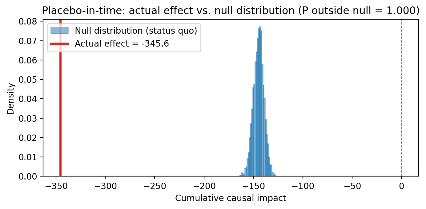
How to read this output. The placebo-in-time check reports several key pieces of information:
Fold summaries. Each fold shifts the treatment time backward into the pre-period. The
meanandsdfor each fold represent the posterior cumulative impact when no real intervention occurred — these are the “null” effects. They should be close to zero if the SC model fits the pre-period well.Hierarchical status-quo model. The
muandtauparameters characterise the learned null distribution:muis the average placebo effect (ideally near zero) andtauis the between-fold variability.P(actual outside null). The key statistic — what fraction of null-distribution draws are smaller in magnitude than the actual estimated effect. A high value (above the threshold, typically 0.95) means the actual effect is clearly distinguishable from the null, supporting the causal claim. A low value means the actual effect looks similar to what arises from noise alone.
SUPPORTED / NOT SUPPORTED. The overall verdict based on whether the probability exceeds the threshold.
Show code cell source
fig, ax = PlaceboInTime.plot(pit_result)
Leave-one-out robustness#
The leave-one-out test removes each donor state in turn and re-estimates the SC, checking whether the effect estimate remains stable. Abadie et al. [2010] and Abadie et al. [2015] recommend this as a standard robustness check. If the estimated effect changes dramatically when a single state is removed, the result is fragile — it depends on one state’s idiosyncratic trajectory rather than the weighted combination. This test is the empirical complement to the weight concentration metric from the design phase: a high concentration score warns that LOO sensitivity is likely.
Note
With 38 donors, CausalPy only drops donors that received non-negligible weight in the original fit — states with near-zero weight have no effect on the synthetic control and don’t need testing.
from causalpy.checks import LeaveOneOut

loo_check = LeaveOneOut()
loo_result = loo_check.run(result, context)
Show code cell output
Initializing NUTS using jitter+adapt_diag...
Multiprocess sampling (4 chains in 4 jobs)
NUTS: [beta, y_hat_sigma]
Sampling 4 chains for 1_000 tune and 1_000 draw iterations (4_000 + 4_000 draws total) took 6 seconds.
Sampling: [beta, y_hat, y_hat_sigma]
Sampling: [y_hat]
Sampling: [y_hat]
Sampling: [y_hat]
Sampling: [y_hat]
Initializing NUTS using jitter+adapt_diag...
Multiprocess sampling (4 chains in 4 jobs)
NUTS: [beta, y_hat_sigma]
Sampling 4 chains for 1_000 tune and 1_000 draw iterations (4_000 + 4_000 draws total) took 7 seconds.
There was 1 divergence after tuning. Increase `target_accept` or reparameterize.
Sampling: [beta, y_hat, y_hat_sigma]
Sampling: [y_hat]
Sampling: [y_hat]
Sampling: [y_hat]
Sampling: [y_hat]
Initializing NUTS using jitter+adapt_diag...
Multiprocess sampling (4 chains in 4 jobs)
NUTS: [beta, y_hat_sigma]
Sampling 4 chains for 1_000 tune and 1_000 draw iterations (4_000 + 4_000 draws total) took 6 seconds.
Sampling: [beta, y_hat, y_hat_sigma]
Sampling: [y_hat]
Sampling: [y_hat]
Sampling: [y_hat]
Sampling: [y_hat]
Initializing NUTS using jitter+adapt_diag...
Multiprocess sampling (4 chains in 4 jobs)
NUTS: [beta, y_hat_sigma]
Sampling 4 chains for 1_000 tune and 1_000 draw iterations (4_000 + 4_000 draws total) took 7 seconds.
Sampling: [beta, y_hat, y_hat_sigma]
Sampling: [y_hat]
Sampling: [y_hat]
Sampling: [y_hat]
Sampling: [y_hat]
Initializing NUTS using jitter+adapt_diag...
Multiprocess sampling (4 chains in 4 jobs)
NUTS: [beta, y_hat_sigma]
Sampling 4 chains for 1_000 tune and 1_000 draw iterations (4_000 + 4_000 draws total) took 6 seconds.
Sampling: [beta, y_hat, y_hat_sigma]
Sampling: [y_hat]
Sampling: [y_hat]
Sampling: [y_hat]
Sampling: [y_hat]
Initializing NUTS using jitter+adapt_diag...
Multiprocess sampling (4 chains in 4 jobs)
NUTS: [beta, y_hat_sigma]
Sampling 4 chains for 1_000 tune and 1_000 draw iterations (4_000 + 4_000 draws total) took 7 seconds.
There was 1 divergence after tuning. Increase `target_accept` or reparameterize.
Sampling: [beta, y_hat, y_hat_sigma]
Sampling: [y_hat]
Sampling: [y_hat]
Sampling: [y_hat]
Sampling: [y_hat]
Initializing NUTS using jitter+adapt_diag...
Multiprocess sampling (4 chains in 4 jobs)
NUTS: [beta, y_hat_sigma]
Sampling 4 chains for 1_000 tune and 1_000 draw iterations (4_000 + 4_000 draws total) took 6 seconds.
Sampling: [beta, y_hat, y_hat_sigma]
Sampling: [y_hat]
Sampling: [y_hat]
Sampling: [y_hat]
Sampling: [y_hat]
Initializing NUTS using jitter+adapt_diag...
Multiprocess sampling (4 chains in 4 jobs)
NUTS: [beta, y_hat_sigma]
Sampling 4 chains for 1_000 tune and 1_000 draw iterations (4_000 + 4_000 draws total) took 7 seconds.
Sampling: [beta, y_hat, y_hat_sigma]
Sampling: [y_hat]
Sampling: [y_hat]
Sampling: [y_hat]
Sampling: [y_hat]
Initializing NUTS using jitter+adapt_diag...
Multiprocess sampling (4 chains in 4 jobs)
NUTS: [beta, y_hat_sigma]
Sampling 4 chains for 1_000 tune and 1_000 draw iterations (4_000 + 4_000 draws total) took 6 seconds.
Sampling: [beta, y_hat, y_hat_sigma]
Sampling: [y_hat]
Sampling: [y_hat]
Sampling: [y_hat]
Sampling: [y_hat]
Initializing NUTS using jitter+adapt_diag...
Multiprocess sampling (4 chains in 4 jobs)
NUTS: [beta, y_hat_sigma]
Sampling 4 chains for 1_000 tune and 1_000 draw iterations (4_000 + 4_000 draws total) took 6 seconds.
Sampling: [beta, y_hat, y_hat_sigma]
Sampling: [y_hat]
Sampling: [y_hat]
Sampling: [y_hat]
Sampling: [y_hat]
Initializing NUTS using jitter+adapt_diag...
Multiprocess sampling (4 chains in 4 jobs)
NUTS: [beta, y_hat_sigma]
Sampling 4 chains for 1_000 tune and 1_000 draw iterations (4_000 + 4_000 draws total) took 6 seconds.
There was 1 divergence after tuning. Increase `target_accept` or reparameterize.
Sampling: [beta, y_hat, y_hat_sigma]
Sampling: [y_hat]
Sampling: [y_hat]
Sampling: [y_hat]
Sampling: [y_hat]
Initializing NUTS using jitter+adapt_diag...
Multiprocess sampling (4 chains in 4 jobs)
NUTS: [beta, y_hat_sigma]
Sampling 4 chains for 1_000 tune and 1_000 draw iterations (4_000 + 4_000 draws total) took 6 seconds.
Sampling: [beta, y_hat, y_hat_sigma]
Sampling: [y_hat]
Sampling: [y_hat]
Sampling: [y_hat]
Sampling: [y_hat]
Initializing NUTS using jitter+adapt_diag...
Multiprocess sampling (4 chains in 4 jobs)
NUTS: [beta, y_hat_sigma]
Sampling 4 chains for 1_000 tune and 1_000 draw iterations (4_000 + 4_000 draws total) took 6 seconds.
There was 1 divergence after tuning. Increase `target_accept` or reparameterize.
Sampling: [beta, y_hat, y_hat_sigma]
Sampling: [y_hat]
Sampling: [y_hat]
Sampling: [y_hat]
Sampling: [y_hat]
Initializing NUTS using jitter+adapt_diag...
Multiprocess sampling (4 chains in 4 jobs)
NUTS: [beta, y_hat_sigma]
Sampling 4 chains for 1_000 tune and 1_000 draw iterations (4_000 + 4_000 draws total) took 6 seconds.
Sampling: [beta, y_hat, y_hat_sigma]
Sampling: [y_hat]
Sampling: [y_hat]
Sampling: [y_hat]
Sampling: [y_hat]
Initializing NUTS using jitter+adapt_diag...
Multiprocess sampling (4 chains in 4 jobs)
NUTS: [beta, y_hat_sigma]
Sampling 4 chains for 1_000 tune and 1_000 draw iterations (4_000 + 4_000 draws total) took 6 seconds.
Sampling: [beta, y_hat, y_hat_sigma]
Sampling: [y_hat]
Sampling: [y_hat]
Sampling: [y_hat]
Sampling: [y_hat]
Initializing NUTS using jitter+adapt_diag...
Multiprocess sampling (4 chains in 4 jobs)
NUTS: [beta, y_hat_sigma]
Sampling 4 chains for 1_000 tune and 1_000 draw iterations (4_000 + 4_000 draws total) took 8 seconds.
Sampling: [beta, y_hat, y_hat_sigma]
Sampling: [y_hat]
Sampling: [y_hat]
Sampling: [y_hat]
Sampling: [y_hat]
Initializing NUTS using jitter+adapt_diag...
Multiprocess sampling (4 chains in 4 jobs)
NUTS: [beta, y_hat_sigma]
Sampling 4 chains for 1_000 tune and 1_000 draw iterations (4_000 + 4_000 draws total) took 7 seconds.
Sampling: [beta, y_hat, y_hat_sigma]
Sampling: [y_hat]
Sampling: [y_hat]
Sampling: [y_hat]
Sampling: [y_hat]
Initializing NUTS using jitter+adapt_diag...
Multiprocess sampling (4 chains in 4 jobs)
NUTS: [beta, y_hat_sigma]
Sampling 4 chains for 1_000 tune and 1_000 draw iterations (4_000 + 4_000 draws total) took 6 seconds.
Sampling: [beta, y_hat, y_hat_sigma]
Sampling: [y_hat]
Sampling: [y_hat]
Sampling: [y_hat]
Sampling: [y_hat]
Initializing NUTS using jitter+adapt_diag...
Multiprocess sampling (4 chains in 4 jobs)
NUTS: [beta, y_hat_sigma]
Sampling 4 chains for 1_000 tune and 1_000 draw iterations (4_000 + 4_000 draws total) took 7 seconds.
Sampling: [beta, y_hat, y_hat_sigma]
Sampling: [y_hat]
Sampling: [y_hat]
Sampling: [y_hat]
Sampling: [y_hat]
Initializing NUTS using jitter+adapt_diag...
Multiprocess sampling (4 chains in 4 jobs)
NUTS: [beta, y_hat_sigma]
Sampling 4 chains for 1_000 tune and 1_000 draw iterations (4_000 + 4_000 draws total) took 6 seconds.
Sampling: [beta, y_hat, y_hat_sigma]
Sampling: [y_hat]
Sampling: [y_hat]
Sampling: [y_hat]
Sampling: [y_hat]
Initializing NUTS using jitter+adapt_diag...
Multiprocess sampling (4 chains in 4 jobs)
NUTS: [beta, y_hat_sigma]
Sampling 4 chains for 1_000 tune and 1_000 draw iterations (4_000 + 4_000 draws total) took 6 seconds.
There were 3 divergences after tuning. Increase `target_accept` or reparameterize.
Sampling: [beta, y_hat, y_hat_sigma]
Sampling: [y_hat]
Sampling: [y_hat]
Sampling: [y_hat]
Sampling: [y_hat]
Initializing NUTS using jitter+adapt_diag...
Multiprocess sampling (4 chains in 4 jobs)
NUTS: [beta, y_hat_sigma]
Sampling 4 chains for 1_000 tune and 1_000 draw iterations (4_000 + 4_000 draws total) took 6 seconds.
There was 1 divergence after tuning. Increase `target_accept` or reparameterize.
Sampling: [beta, y_hat, y_hat_sigma]
Sampling: [y_hat]
Sampling: [y_hat]
Sampling: [y_hat]
Sampling: [y_hat]
Initializing NUTS using jitter+adapt_diag...
Multiprocess sampling (4 chains in 4 jobs)
NUTS: [beta, y_hat_sigma]
Sampling 4 chains for 1_000 tune and 1_000 draw iterations (4_000 + 4_000 draws total) took 7 seconds.
Sampling: [beta, y_hat, y_hat_sigma]
Sampling: [y_hat]
Sampling: [y_hat]
Sampling: [y_hat]
Sampling: [y_hat]
Initializing NUTS using jitter+adapt_diag...
Multiprocess sampling (4 chains in 4 jobs)
NUTS: [beta, y_hat_sigma]
Sampling 4 chains for 1_000 tune and 1_000 draw iterations (4_000 + 4_000 draws total) took 6 seconds.
Sampling: [beta, y_hat, y_hat_sigma]
Sampling: [y_hat]
Sampling: [y_hat]
Sampling: [y_hat]
Sampling: [y_hat]
Initializing NUTS using jitter+adapt_diag...
Multiprocess sampling (4 chains in 4 jobs)
NUTS: [beta, y_hat_sigma]
Sampling 4 chains for 1_000 tune and 1_000 draw iterations (4_000 + 4_000 draws total) took 6 seconds.
Sampling: [beta, y_hat, y_hat_sigma]
Sampling: [y_hat]
Sampling: [y_hat]
Sampling: [y_hat]
Sampling: [y_hat]
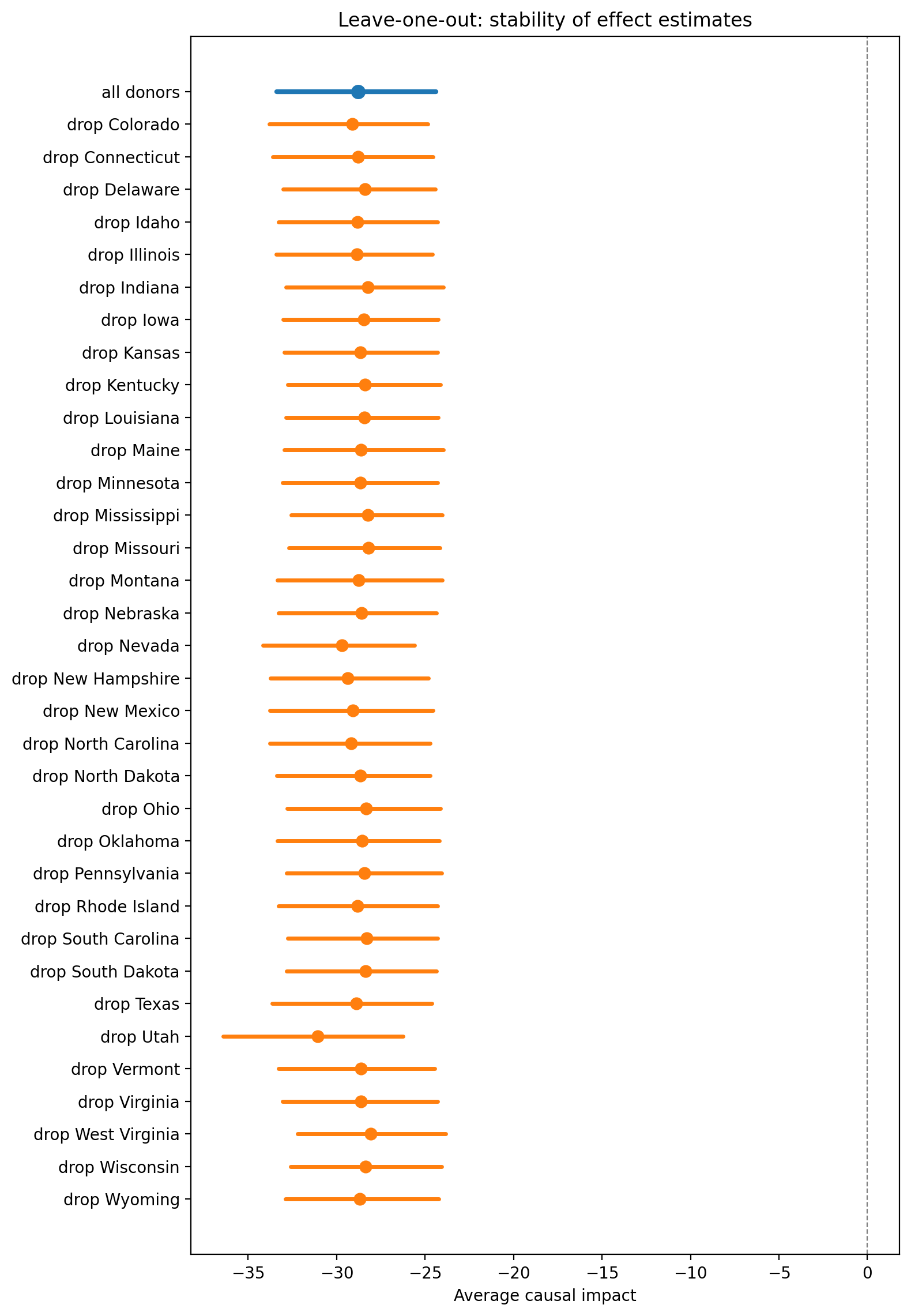
print(loo_result.text)
Leave-one-out analysis: dropped each of 34 control units. Examine the table for consistency of effect estimates.
loo_result.table
| dropped_unit | mean | median | hdi_lower | hdi_upper | p_gt_0 | relative_mean | relative_hdi_lower | relative_hdi_upper | |
|---|---|---|---|---|---|---|---|---|---|
| 0 | Colorado | -29.101407 | -28.967615 | -33.821216 | -24.840250 | 0.0 | -32.487218 | -35.914601 | -29.158560 |
| 1 | Connecticut | -28.800733 | -28.633307 | -33.613685 | -24.564442 | 0.0 | -32.260663 | -35.805540 | -28.964884 |
| 2 | Delaware | -28.394817 | -28.211391 | -33.040408 | -24.439636 | 0.0 | -31.953253 | -35.378803 | -28.823849 |
| 3 | Idaho | -28.827627 | -28.718432 | -33.274242 | -24.304701 | 0.0 | -32.280386 | -35.609735 | -28.782588 |
| 4 | Illinois | -28.870066 | -28.763831 | -33.427057 | -24.598069 | 0.0 | -32.314717 | -35.856374 | -29.180495 |
| 5 | Indiana | -28.248664 | -28.115591 | -32.854411 | -23.954791 | 0.0 | -31.839643 | -35.397702 | -28.589315 |
| 6 | Iowa | -28.466815 | -28.387968 | -33.033032 | -24.254081 | 0.0 | -32.006185 | -35.373698 | -28.667744 |
| 7 | Kansas | -28.650270 | -28.524542 | -32.955512 | -24.300882 | 0.0 | -32.148216 | -35.320006 | -28.707181 |
| 8 | Kentucky | -28.392105 | -28.297762 | -32.750642 | -24.119890 | 0.0 | -31.951633 | -35.177676 | -28.554424 |
| 9 | Louisiana | -28.443421 | -28.341902 | -32.879347 | -24.244657 | 0.0 | -31.991321 | -35.267164 | -28.659797 |
| 10 | Maine | -28.621918 | -28.527061 | -32.947105 | -23.951757 | 0.0 | -32.124699 | -35.859357 | -28.995017 |
| 11 | Minnesota | -28.656880 | -28.555374 | -33.051280 | -24.284891 | 0.0 | -32.152366 | -35.386324 | -28.693711 |
| 12 | Mississippi | -28.239665 | -28.096322 | -32.575452 | -24.034060 | 0.0 | -31.834459 | -35.055468 | -28.481754 |
| 13 | Missouri | -28.200431 | -28.054990 | -32.715081 | -24.169818 | 0.0 | -31.803237 | -35.152906 | -28.596628 |
| 14 | Montana | -28.761032 | -28.648315 | -33.351882 | -24.041424 | 0.0 | -32.227656 | -35.884187 | -28.799678 |
| 15 | Nebraska | -28.580328 | -28.431760 | -33.289494 | -24.373388 | 0.0 | -32.092523 | -35.550699 | -28.768193 |
| 16 | Nevada | -29.702217 | -29.589238 | -34.183157 | -25.585458 | 0.0 | -32.944112 | -36.311074 | -29.947591 |
| 17 | New Hampshire | -29.369824 | -29.294326 | -33.755752 | -24.809967 | 0.0 | -32.689869 | -36.057577 | -29.324422 |
| 18 | New Mexico | -29.076476 | -29.018241 | -33.789780 | -24.558335 | 0.0 | -32.466533 | -36.010535 | -29.055364 |
| 19 | North Carolina | -29.173950 | -29.090835 | -33.769704 | -24.719415 | 0.0 | -32.542292 | -36.056197 | -29.240877 |
| 20 | North Dakota | -28.661781 | -28.560592 | -33.400815 | -24.703200 | 0.0 | -32.157501 | -35.645882 | -29.063117 |
| 21 | Ohio | -28.346684 | -28.213064 | -32.800372 | -24.144223 | 0.0 | -31.916189 | -35.246265 | -28.610996 |
| 22 | Oklahoma | -28.557284 | -28.413305 | -33.364913 | -24.208086 | 0.0 | -32.073126 | -35.615678 | -28.644425 |
| 23 | Pennsylvania | -28.428831 | -28.359437 | -32.823067 | -24.059735 | 0.0 | -31.978831 | -35.479379 | -28.756211 |
| 24 | Rhode Island | -28.809883 | -28.679364 | -33.303477 | -24.278751 | 0.0 | -32.267003 | -35.579699 | -28.712213 |
| 25 | South Carolina | -28.305873 | -28.207955 | -32.781874 | -24.279575 | 0.0 | -31.885024 | -35.199414 | -28.689232 |
| 26 | South Dakota | -28.374424 | -28.254161 | -32.815597 | -24.345651 | 0.0 | -31.938673 | -35.222870 | -28.744866 |
| 27 | Texas | -28.902487 | -28.737193 | -33.642149 | -24.603124 | 0.0 | -32.338683 | -36.068006 | -29.267939 |
| 28 | Utah | -31.087703 | -31.027254 | -36.407041 | -26.249496 | 0.0 | -33.943828 | -37.640983 | -30.325556 |
| 29 | Vermont | -28.615677 | -28.490485 | -33.283191 | -24.457946 | 0.0 | -32.119852 | -35.569926 | -28.866004 |
| 30 | Virginia | -28.639973 | -28.574378 | -33.061977 | -24.299221 | 0.0 | -32.139426 | -35.545744 | -28.876338 |
| 31 | West Virginia | -28.073949 | -27.939191 | -32.217032 | -23.844319 | 0.0 | -31.708125 | -34.908748 | -28.430435 |
| 32 | Wisconsin | -28.362807 | -28.255105 | -32.612559 | -24.057965 | 0.0 | -31.928662 | -35.230223 | -28.659902 |
| 33 | Wyoming | -28.679574 | -28.508818 | -32.881563 | -24.235020 | 0.0 | -32.170552 | -35.462920 | -28.873099 |
How to read this table. Each row shows the effect estimate after dropping a single donor state from the pool. The dropped_unit column identifies which state was excluded; the remaining columns show the causal impact summary from the re-estimated SC. Look for two things:
Stability of point estimates. If the
meancolumn is broadly consistent across rows, the result is not driven by any single donor. Large swings when a particular state is dropped indicate fragility.Consistency of credible intervals. If one row’s HDI includes zero while the others exclude it, the causal claim depends critically on that donor — a red flag.
Donors whose removal causes the largest shifts are typically those receiving the highest weight in the original SC fit. This connects back to the weight concentration metric from the design phase: a donor pool with more evenly distributed weights is less vulnerable to LOO perturbations.
Show code cell source
fig, ax = LeaveOneOut.plot(loo_result, baseline_stats=stats)
Prior sensitivity#
For Bayesian SC, it is important to check that the posterior effect estimates are not unduly driven by the prior specification. Kim et al. [2020] discuss prior specification for Bayesian synthetic control and recommend checking sensitivity to prior choices — a standard practice in Bayesian inference [Gelman et al., 2013]. The PriorSensitivity check re-fits the model with alternative prior specifications and compares the resulting effect summaries. If conclusions shift substantially under different priors, the data may not be informative enough to support the causal claim independently of the prior.
from causalpy.checks import PriorSensitivity

n_donors = len(control_units)
y_hat_prior = Prior(
    "Normal",
    sigma=Prior("HalfNormal", sigma=10, dims=["treated_units"]),
    dims=["obs_ind", "treated_units"],
)

prior_check = PriorSensitivity(
    alternatives=[
        {
            "name": "diffuse (conc=0.5)",
            "model": cp.pymc_models.WeightedSumFitter(
                priors={
                    "beta": Prior(
                        "Dirichlet",
                        a=np.ones(n_donors) * 0.5,
                        dims=["treated_units", "coeffs"],
                    ),
                    "y_hat": y_hat_prior,
                },
                sample_kwargs={"target_accept": 0.95, "random_seed": seed},
            ),
        },
        {
            "name": "concentrated (conc=10)",
            "model": cp.pymc_models.WeightedSumFitter(
                priors={
                    "beta": Prior(
                        "Dirichlet",
                        a=np.ones(n_donors) * 10,
                        dims=["treated_units", "coeffs"],
                    ),
                    "y_hat": y_hat_prior,
                },
                sample_kwargs={"target_accept": 0.95, "random_seed": seed},
            ),
        },
    ]
)
prior_result = prior_check.run(result, context)
print(prior_result.text)
Initializing NUTS using jitter+adapt_diag...
Multiprocess sampling (4 chains in 4 jobs)
NUTS: [beta, y_hat_sigma]
Sampling 4 chains for 1_000 tune and 1_000 draw iterations (4_000 + 4_000 draws total) took 17 seconds.
There were 4 divergences after tuning. Increase `target_accept` or reparameterize.
Sampling: [beta, y_hat, y_hat_sigma]
Sampling: [y_hat]
Sampling: [y_hat]
Sampling: [y_hat]
Sampling: [y_hat]
Initializing NUTS using jitter+adapt_diag...
Multiprocess sampling (4 chains in 4 jobs)
NUTS: [beta, y_hat_sigma]
Sampling 4 chains for 1_000 tune and 1_000 draw iterations (4_000 + 4_000 draws total) took 4 seconds.
Sampling: [beta, y_hat, y_hat_sigma]
Sampling: [y_hat]
Sampling: [y_hat]
Sampling: [y_hat]
Sampling: [y_hat]
Prior sensitivity analysis: compared 2 alternative prior specifications.
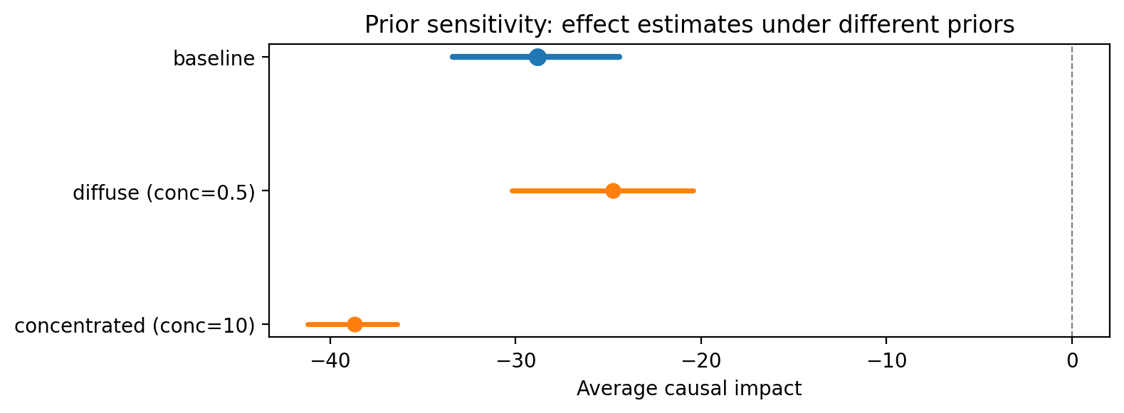
prior_result.table
| prior_spec | mean | median | hdi_lower | hdi_upper | p_gt_0 | relative_mean | relative_hdi_lower | relative_hdi_upper | |
|---|---|---|---|---|---|---|---|---|---|
| 0 | diffuse (conc=0.5) | -24.757090 | -24.398877 | -30.184998 | -20.415986 | 0.0 | -29.023331 | -33.340695 | -25.277951 |
| 1 | concentrated (conc=10) | -38.685402 | -38.671872 | -41.216119 | -36.365544 | 0.0 | -39.052369 | -40.580579 | -37.600516 |
How to read these results. Each row shows the effect summary under a different Dirichlet concentration parameter for the donor weights. Compare across rows: if the point estimates and intervals are broadly consistent, the conclusions are robust to prior choice. If they diverge — particularly if one specification produces a credible interval that includes zero while another excludes it — the data may not be informative enough to support the causal claim independently of the prior.
Show code cell source
fig, ax = PriorSensitivity.plot(
    prior_result, baseline_stats=stats, baseline_label="baseline (conc=1)"
)
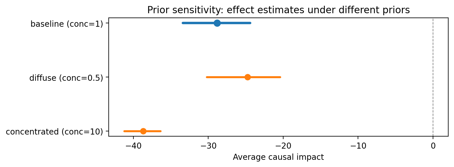
Running all checks in a pipeline#
The checks above were run individually for exposition. In practice, CausalPy’s SensitivityAnalysis pipeline step can run all applicable checks in a single call, accumulating results into a SensitivitySummary. Combined with EstimateEffect, this gives a reproducible end-to-end workflow:
from causalpy.steps.sensitivity import SensitivityAnalysis

sensitivity = SensitivityAnalysis(
    checks=[
        PlaceboInSpace(),
        LeaveOneOut(),
    ]
)
context_with_sensitivity = sensitivity.run(context)

for check_result in context_with_sensitivity.sensitivity_results:
    print(f"--- {check_result.check_name} ---")
    print(check_result.text)
See the Pipeline Workflow notebook for a full walkthrough of CausalPy’s pipeline API, including how to chain EstimateEffect, SensitivityAnalysis, and GenerateReport into a single reproducible pipeline.
Which checks matter most in your setting?#
The four robustness checks above probe different failure modes, and their relative importance depends on your data structure:
Few donor units? The leave-one-out test may reveal that one unit drives the entire result. Consider augmented SC [Ben-Michael et al., 2021] as a remedy. (With 38 states in the Proposition 99 example, this is less of a concern.)
Short pre-period? The placebo-in-time test helps gauge whether the model has enough pre-treatment data to learn stable donor weights, while a longer pre-period improves asymptotic properties [Ferman, 2021]. The 19-year pre-period here is reasonably long for annual data.
Uncertain priors? If you are using diffuse priors on a sparse donor pool, the prior sensitivity check reveals whether your Bayesian conclusions are data-driven or prior-dominated.
Strong result? A placebo-in-space test that shows your effect is larger than all placebo effects provides the strongest permutation-based evidence for a causal claim [Abadie et al., 2010]. For the Proposition 99 analysis, Abadie et al. [2010] found that California’s effect was an extreme outlier relative to placebo states.
Putting it together: what did these checks tell us?#
Each design and post-experiment check probes the SC fit from a different angle. Here is what we observed for this Prop 99 analysis (consult the relevant cell above for the actual numbers, since they may shift on re-execution):
Donor pool: mostly low-to-negative pre-treatment correlations with California; many candidate donors flagged for exclusion. (See the donor-correlation diagnostics above.)
Power curve: detection rate rises with effect size and crosses 80% at a moderate magnitude. (See the power-curve plot above.)
Placebo-in-time sanity check (design phase): recovered mean strongly negative, 94% HDI excludes zero — a clear failure. (See the rehearsal summary above.)
Post-experiment fit: California diverges sharply downward from its synthetic counterpart after 1989. (See the impact plot above.)
Placebo-in-space: California’s effect is compared against the donor placebo distribution. (See the
pis_resultranking and plot above.)Placebo-in-time (post-experiment): placebo intervention dates in the pre-period are checked for spurious effects. (See the post-experiment placebo-in-time output above.)
Leave-one-out: point estimate’s stability is checked when each donor is dropped. (See the leave-one-out plot above.)
Prior sensitivity: the posterior’s robustness to alternative priors is reported. (See the prior-sensitivity output above.)
The central tension#
The power curve looks healthy: at moderate effect sizes the design appears comfortably powered. Yet validate_design(injected_effect=0) returns a strongly negative recovered mean with the 94% HDI excluding zero — a placebo-in-time failure at the design stage. The mechanism is straightforward: the donor pool cannot reproduce California’s trajectory shape across the full pre-period, so the synthetic control’s point estimate is biased even before any real intervention is considered.
Pre-period only, or full-data too?#
It is tempting to wave away the design-phase failure as an artefact of the truncated pseudo-pre / pseudo-post split. We should resist that temptation. The same extrapolation bias that mis-predicts the pseudo-post window is highly likely to persist into the 1989–2000 estimation window, which means:
Magnitude estimation (how big was Prop 99’s effect?) is probably biased by this mechanism. The headline cumulative-impact number from the post-experiment fit should be read with that bias in mind.
Existence-of-effect inference (was there an effect at all?) rests on firmer ground. The placebo-in-space test is permutation-based: its validity does not require the SC point estimate to be unbiased, only that California’s post/pre RMSPE ratio is an outlier relative to the donor placebo distribution. Look at the
pis_resultranking and plot above and judge for yourself whether California sits cleanly outside that distribution; if it does, the existence claim survives the design-phase bias.
Put differently: the post-experiment placebo-in-space check provides inference that is robust to the very bias the design-phase placebo-in-time uncovered.
Alternative methods to consider#
If the magnitude question matters (e.g. for cost–benefit work), several SC variants handle this kind of trajectory-shape mismatch better than the vanilla weighted sum:
Time-trend-augmented synthetic control, which adds a unit-specific linear or smooth trend to absorb shape mis-match.
Synthetic difference-in-differences [], which combines DiD’s parallel-trend assumption with SC’s donor weighting.
Augmented synthetic control [Ben-Michael et al., 2021], which uses an outcome model to bias-correct the SC weights.
These are pointers, not endorsements; choosing among them requires its own diagnostics on the same dataset.
Reflection#
Which of the failure modes seen in this notebook would you expect to see in a synthetic control analysis from your own work? For example:
A retailer measuring the effect of a regional promotion against other regions: does the treated region have a trajectory shape (seasonality, growth rate) that the donor regions can reproduce, or is it idiosyncratic?
A health-policy analysis comparing one country’s outcome under a new regulation against peer countries: do the peers track the treated country’s pre-period closely, or are there obvious shape mismatches that point at omitted structural factors?
Running validate_design(injected_effect=0) on your own design before looking at the post-treatment data is a cheap way to surface this kind of structural issue while there is still time to widen the donor pool, switch methods, or downgrade the analysis from “estimate magnitude” to “test existence”.